Multivariate Linear Regression detailed explanation

In the previous post, Simple Linear Regression detailed Explanation we understand how to apply Linear Regression to the problem statement where we have only one independent variable. However, in the real-time scenario, there will be many independent variables that will contribute to predicting the target variable. Here, I will be demonstrating using the Boston dataset from the sklearn library.

Let's create the Boston dataset and split it into the training and test datasets for evaluation. The dataset has 12 independent variables and 1 dependent variable or target variable.

import pandas as pd
from sklearn.datasets import load_boston

boston = load_boston()
data = pd.DataFrame(boston.data,columns=boston.feature_names)
data['price'] = pd.Series(boston.target)

y = data.pop('price').values
X = data.values

# Splitting dataset into test and train
X_train, X_test, y_train, y_test = train_test_split(X, y, test_size = 0.33, random_state = 5)

Recap

We started defining what Linear Regression is. We defined metrics like ESS, RSS, TSS, RSE, and R squared that help us to find the best-fit line and evaluate model performance. After deep understanding, we defined the cost function and used various techniques to minimize it:

1. Ordinary Least Square - OLS Estimator
2. Mean Square Error - MSE

that can be used to find the best-fit line. We defined a Python function to calculate OLS. Thereafter we defined the MSE function and understood the concept of Gradient Descent that is used to minimize MSE. We discussed three different types of gradient descent approaches:

1. Batch Gradient Descent
2. Stochastic Gradient Descent
3. Mini Batch Gradient Descent

While understanding the above concepts we also learned about the sklearn packages LinearRegression and SGDRegressor which use OLS and Stochastic Gradient Descent approaches respectively to find the best fit line. We have discussed this with a single variable as an independent variable.

Multivariate Linear Regression (MLR)

Multivariate Linear Regression is the regression where we find the best-fit plane instead of the line to explain more than one independent variable. In other words, we can say Multivariate Linear Regression is the extension of the Simple Linear Regression.

Multivariate Linear Regression is given by the equation:

$$ y = \beta_0 + \beta_1x_1 + \beta_2x_2 + . . . . . + \beta_nx_n + \epsilon$$

Similar to the Simple Linear Regression (SLR) model, the Multivariate Linear Regression (MLR) model also has a cost function associated with it. And we need to minimize the cost function using the Gradient Descent Algorithm. The formula of the cost function is represented as:

$$ J(\theta_1, \theta_2, \theta_3, . . . , \theta_n) = {1\over 2m} \sum_{i = 1}^m{(h_\theta(x^{(i)}) - y^{(i)})}^2$$

As we can see the cost function is similar to the MSE cost function which we discussed in Simple Linear Regression. And here instead of converging two coefficients theta 1 and theta 2. We have to converge n + 1 coefficients where n represents the number of features and an intercept. The gradient descent of multivariate linear regression is represented as:

$$\theta_0 = \theta_0 - \alpha{1 \over m} \sum_{i = 1}^m{(h_\theta(x^{(i)}) - y^{(i)})}.x_0^{(i)}$$

$$\theta_1 = \theta_1 - \alpha{1 \over m} \sum_{i = 1}^m{(h_\theta(x^{(i)}) - y^{(i)})}.x_1^{(i)}$$

$$\theta_2 = \theta_2 - \alpha{1 \over m} \sum_{i = 1}^m{(h_\theta(x^{(i)}) - y^{(i)})}.x_2^{(i)}$$

And so on for all of the thetas. Also, we repeat the above steps until we reach convergence.

NOTE: It's not possible to show diagram of more than 2 or 3 dimension on the paper. Here we need to fit the n dimensional plane to find the best model. 

Moving from SLR to MLR

We have learned about Simple Linear Regression in the previous post. Let's see what remains the same and what are the complication added to moving to MLR from SLR.

What remains the same:

1. The assumptions that we have talked about remain the same. i.e. Linearity, Constant Error Variance, Independent Error Terms, Normal Errors, No multicollinearity, and Exogeneity.
2. Coefficients of the Regression curve are obtained by minimizing the cost function using Gradient Descent.

What new:

1. The model now fits the hyperplane instead of the line
2. Overfitting
3. Multicollinearity
4. Feature Selection
5. Feature Scaling

Let's discuss what has changed moving from SLR to MLR in detail.

From Line to Hyperplane

As we have seen earlier to find the best fit for the model we used to find the line that explains the target variable. But now as we have more than one independent variable we need to draw a hyperplane to explain the target variable. The hyperplane is drawn in n dimension space where n is the number of independent variables used to generate the model.

Overfitting

As we keep on adding the independent variables, the model may become too complex and there is a high possibility that the model memorizes the training data or sample data and will fail to generalize the test data or population dataset. 

To identify overfitting we find the accuracy of the model on the test and training data set. And if the difference between the accuracy of the test and training data is huge we can conclude that the model has overfitted and fails to generalize on the test dataset.

Let's create a basic Linear Regression using all of the 12 features.

lm = LinearRegression()
lm.fit(X_train, y_train)

We have a model with us trained on 12 features available. Let's calculate the r2 score (as it explains the strength of the model) for both test and training datasets.

y_pred_test = lm.predict(X_test)
y_pred_train = lm.predict(X_train)

print(r2_score(y_test, y_pred_test))
print(r2_score(y_train, y_pred_train))

# Output
0.6955388005506375
0.7551332741779997

From the output, we can observe that the difference in r2 score between training and test datasets is about 6%. Therefore stating that our model has learned and failed to generalize on the test dataset. This is happening because of overfitting.

NOTE: We should always try to find high accuracy with keeping the model simple and should be able to tell the story from the model in the business perspective.

Multicollinearity

Multicollinearity refers to the phenomenon of having related predictor variables(i.e. independent variables) in the input dataset.

In simple terms, a model that has been built using several independent variables, some of these variables might be interrelated, due to which the presence of that variable in the model is redundant. There are various ways to deal with multicollinearity:

1. Pairwise correlations
2. Variance Inflation Factor

Pairwise correlations

Looking at the correlation between different pairs of independent variables. Pandas provide the df.corr() function to find the pairwise correlation. Let's look into the example shown below:

correlation = data.corr()

We can plot the heat map for the visualizing the values:

plt.figure(figsize=(12,8))
sns.heatmap(correlation, annot=True)
plt.show()

OUTPUT:

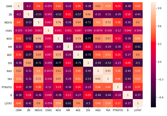
Once we correlate plotted we can go ahead and remove highly correlated values. But note that business knowledge is needed so that we don't remove any feature that may impact the business.

Variance Inflation Factor

Sometimes instead of just one variable, the independent variable might depend upon a combination of other variables. VIF calculates how well one independent variable is explained by all the other independent variables combined excluding the target variable.

$$VIF_i = {1 \over 1 - R_i^2} $$

To calculate R R-squared value for the feature we select the feature and regress it against all other independent variables.

The common heuristic we follow for the VIF values is:

• > 10: high VIF value and the variable should be eliminated. (As it denotes that column is highly correlated)
• > 5:  Can be okay, but it is worth inspecting. (As it denotes that column is moderately correlated)
• < 5: Good VIF value. No need to eliminate this variable. (As it denotes that column is almost not correlated)

Let's see how we can calculate VIF using Python:

from statsmodels.stats.outliers_influence import variance_inflation_factor
import pandas as pd

vif = pd.DataFrame()
vif['Features'] = X_train.columns
vif['VIF'] = [variance_inflation_factor(X_train.values, i) for i in range(X_train.shape[1])]
vif['VIF'] = round(vif['VIF'], 2)
vif = vif.sort_values(by = "VIF", ascending = False)
print(vif)

OUTPUT:

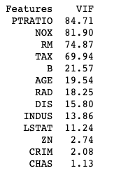
Here in the code shown above, we are calculating VIF for every column of the dataset using variance_inflation_factor function.

We understand what is multicollinearity and how to detect it in the model. If we find that we have multicollinearity in the model, we need to deal with it. Below are the methods to deal with the multicollinearity:

1. Dropping variables
2. Create a new variable
3. Add interaction features: Features derived using some of the original features
4. Variable transformations:
   • Principal component analysis (PCA)
   • Partial least squares (PLS)

Dropping variables

Dropping a variable is straightforward where we drop highly correlated (positive correlated or negative correlated) features from the dataset.

Create a new variable

We can also create new derived variables from the existing variables. E.g. Consider a dataset where we have the height and weight of the person where height and weight and highly correlated.

We create a derived variable BMI which is Weight/height and delete the weight and height column from the dataset.

Interaction Term

Interaction effects occur when the effect of one variable depends on the value of another variable.

In more complex study areas, the independent variables might interact with each other. Interaction effects indicate that a third variable influences the relationship between an independent and dependent variable. This type of effect makes the model more complex, but if the real world behaves this way, it is critical to incorporate it into your model.

There can be an interaction between categorical variables or between continuous variables. Let's understand them intuitively.

Interaction between the categorical variable

Consider a scenario where the taste of food depends on the type of food and condiment. Here, independent categorical variables are food and condiments. And the dependent variable is enjoyment.

Satisfaction = Food * Condiment

Satisfaction depends on the Food and Condiment, so individually we will not be able to conclude to correct results. And we can figure out the interaction term using an interaction plot.

The crossed lines on the graph suggest that there is an interaction effect, which can be confirmed using a significant p-value for the Food*Condiment term. Parallel lines indicate that there is no interaction effect.

Interaction between the continuous variables

Similar to an interaction term in categorical variables, we can generate an interaction term for the continuous variables. Consider a scenario where we have continuous independent variables processing time, temperature, and pressure. The dependent variable is the strength of the product.

Here we can generate a feature: temperature*pressure as an interaction term and the feature is found to have having significant p-value.

Here also we can figure out the interaction effect using an interaction plot.

NOTE: 

1. While the plots help you interpret the interaction effects, use a hypothesis test to determine whether the effect is statistically significant.
2. You can have higher-order interactions. Three-way interaction has three variables in the term, such as Food*Condiment*X. However, this type of effect is challenging to interpret. In practice, analysts use them infrequently. 

Variable transformations

To know about Variable Transformations please refer to the post: Dimension Reduction Techniques in Python.

Feature Selection

This is one of the crucial aspects of multiple linear regression. By now you must have realized the importance of selecting the right feature for the model.

There are two ways to select the features in the model. These are:

1. Manual Feature Elimination
2. Automated Approach
3. Balanced Approach

Manual Feature Elimination is the approach where we manually eliminate the feature to generate the model and increase the accuracy. We can eliminate features using below mentioned approaches:

1. We start will all the features and eliminate the features one by one.
2. We start with a single feature and keeps on adding a new feature to the model

Here, let's consider the first approach where we start with all the features and eliminate less significant features. 

import statsmodels.api as sm

# Step 1: Adding Constant
col = X.columns
X_train_lm = sm.add_constant(X_train[col])

# Step 2
lr = sm.OLS(y_train, X_train_lm).fit()

# Step 3
print(lr.summary())

OUTPUT:

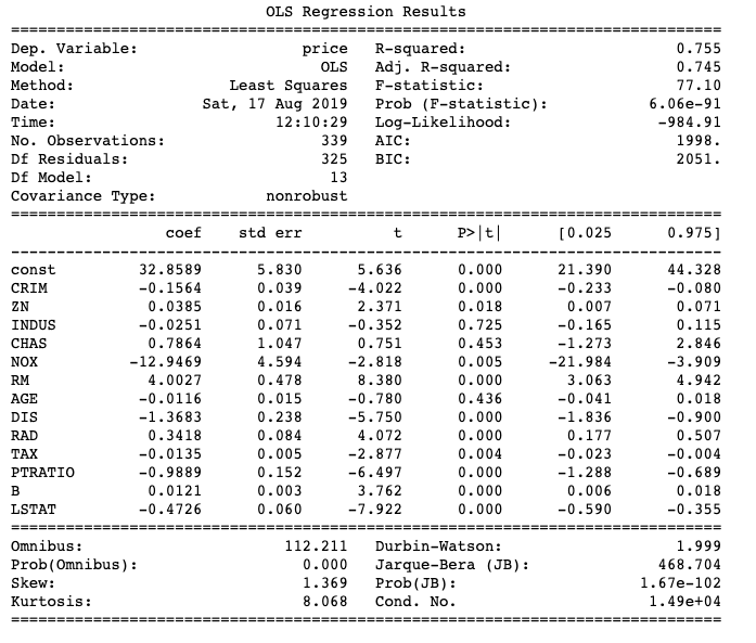
As you have noticed above we are using the OLS method from the stats model instead of LinearRegression from the sklearn package. The reason behind this is that stats models give much more details about statistical reports than sklearn.  Let's see and understand the above code.

1. The first step is to add a constant or an intercept to the dataset. Because the intercept is not included by default.
2. The next step is to train the model using the training dataset.
3. Finally, we can see the statistical report of the features.

NOTE: When we have less number of features suppose 10 then it's possible to do select features manually. But suppose when we have more than 100 features, can we still select features manually?

Automated Approach is the approach where we use algorithms to decide which feature to consider for the model. There are various techniques available:

1. Recursive Feature Elimination (RFE)
2. Forward and backward stepwise selection
3. Lasso Regularization

Recursive Feature Elimination (RFE)

Recursive feature elimination is based on the idea of repeatedly constructing a model and choosing the best or worst-performing feature. During the feature selection, the RFE model is constructed continuously unless all the features are exhausted.

It is a greedy optimization for finding the best-performing subset of features. The RFE algorithm works as:

1. Firstly the model fits all variables.
2. Then it calculates variable coefficients and their importance.
3. It ranks the variable based on the model (In this case linear regression) and then removes the low-ranking variable in each iteration.

Sklearn does the mentioned process automatically if we define the number of features we want to reduce it to. Consider the code shown below demonstrating RFE to select the features for the model:

# Creating sklearn linear regression model on all the features.
lm = LinearRegression()
lm.fit(X_train, y_train)

rfe = RFE(lm, 8)
rfe = rfe.fit(X_train, y_train)

col = X_train.columns[rfe.support_]

X_train_lm = sm.add_constant(X_train[col])
lr = sm.OLS(y_train, X_train_lm).fit()
print(lr.summary())

Forward and backward stepwise selection

In forwarding feature selection:

1. We start with the null model. ( i.e. Model has no independent variable and we have just an intercept and target variable)
2. We pick the best independent variable. (which results in the lowest residual sum of squares)
3. Repeat unless we are satisfied with the results.

The backward selection is the opposite of forwarding selection where,

1. We start with all the variables to build the model.
2. Remove the least significant variable.
3. Repeat unless we are satisfied with the results. (For instance, we may stop when all variables have significant p-values)

By now you might have guessed that RFE is a type of backward stepwise selection.

Lasso Regularization

We learn about it later post. For now, it's important to know that this is also the technique available for feature selection.

Balanced Approach is the combination of both manual and automated approaches. In industry to solve the problem set having 100+ features, we use a combination of both Manual and Automated Feature selection.

Feature Scaling

Feature scaling is the technique to convert all the independent variables to the same scale e.g. -1 to 1. It is a necessary step because Gradient Descent will take more time to find a global minimum if features are not on the same scale. Scaling helps in:

1. Interpretation
2. Gradient descent faster convergence

There are various methods available to scale the features. Popular ones are:

1. Standardization 
2. MinMax Scaling or normalization

Standardization

Standardization brings all of the data into a standard normal distribution with mean zero and standard deviation one.

 \[\text {Standardisation:  $x$} = {x - mean(x) \over sd(x)}\] 

MinMax Scaling

MinMax Scaling or normalization brings all of the data in the range of 0 and 1. This technique is preferred to handle outliers.

NOTE: Scaling doesn't have any effect on the best-fit line. Scaling only affects the coefficient of the best-fit line.

 \[\text {MinMax scaling:  $x$} = {x - min(x) \over max(x) - min(x)}\] 

Model Performance

The R-squared will always either increase or remain the same when you add more variables. Because you already have the predictive power of the previous variable the R-squared value can not go down. And a new variable, no matter how insignificant it might be, cannot decrease the value of R-squared.

So far so good, but how do we compare two models having different counts of features? According to the above statement, R squared will only increase if we add more features. So instead of calculating R squared we calculate adjusted R squared, which is denoted by:

 \[\text {Adjusted  $R^2$} = 1 - {{RSS / (n - k- 1)} \over TSS / (n-1)}\] 

Or, it can be also represented as,

\[\text {Adjusted  $R^2$} = 1 - (1 - R^2){(n-1) \over  (n - k - 1)}\] 

where n - k - 1 is called the degree of freedom n represent the number of observation and k represent the no of independent variables.

Note:

1. As the degree of freedom decreases, R squared will only increase.
2. As k increases, adjusted R squared tend to decrease, if we add useless variables.

Summary

Here we started looking at what changed when we moved from SLR to MLR. We discussed:

1. The model now fits the hyperplane instead of the line
2. Overfitting
3. Multicollinearity
4. Feature Selection
5. Feature Scaling

We concluded with the model performance and introduced adjusted R squared which is an improvement to R squared.