Simple Linear Regression detailed Explanation

In this post, we will be starting to learn about the Linear Regression algorithm. We are starting up with Linear Regression because it is an easy-to-understand but very powerful algorithm to solve machine learning problems. 

We will be doing hands-on as we process along with the post. I will be using the Boston house price dataset from sklearn to explain Linear Regression.

Before we start let's just import the data and create the data frame.

import pandas as pd
from sklearn.datasets import load_boston

boston = load_boston()
data = pd.DataFrame(boston.data,columns=boston.feature_names)
data['price'] = pd.Series(boston.target)
print(data.head())

NOTE: In this post, we will be using only one column:

• RM: Average number of rooms per dwelling

There are different types of regression we can perform depending on the data and outcome we are predicting:

1. Simple Linear Regression: Regression with single independent and target variable
2. Multi Linear Regression: Regression with multiple independent variables

In this post, we will be covering Simple Linear Regression. First, let's get started by defining linear regression.

Linear Regression

Linear regression is a method of finding the best straight-line fit between the dependent variable or target variable and one or more independent variables. In other terms finding the best fit line that tells the relationship between the target variable (Y) and all the independent variables(X).

Here, we will find the best-fit line between price and RM(Average number of rooms per dwelling) column from the Boston data set. The distribution is shown below:

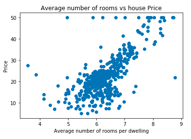
Our goal when solving a linear regression is to find the line also known as a regression line which fits the independent variables in the best way. In this case, since we have only one variable our best-fit line will be:

price = m(RM) + b, where m and b are the variables that we need to fit.

To find the value of m and b, we try with different values and calculate the cost function for each combination. We have two different approaches that we use in Linear Regression and minimization to obtain the best-fit line. These are:

1. Ordinary Least Squares (OLS) Estimators
2. Mean Squared Error (MSE)

Before we move ahead let's focus on one of the data points and understand the terminology that will help us to understand the concept in detail:

Refer to the chart shown below:

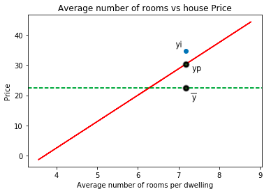
NOTE:

1. Here the solid red line is the best fit line fitted on the dataset.
2. The dotted green line is the average of the target variable
3. yi is one of the observations from the dataset, yp is the predicted value for the observation and y mean is the mean point for the observation.

There are a few metrics that we calculate to find the best-fit line.

ESS: Explained the sum of square

Also known as the Sum of Squares due to Regression (SSR) is the sum of the squares of the deviations of the predicted values from the mean value of a target variable.

NOTE: Don't get confused with the Sum of Squared Residuals. We will learn about it in a while.

It is represented as:

$$SSR = \sum(\hat{Y_i} - \bar{Y})^2$$

RSS: Residual Sum of squares

Also known as the sum of squared residuals (SSR) or the sum of squared errors (SSE) is the sum of the squares of residuals i.e. Deviation from the actual value. It is represented as:

$$SSE = \sum(Y_i - \hat{Y_i})^2$$

TSS: Total Sum of Squares

Also known as SST is defined as the sum of the squares of the difference of the dependent variable and its mean.

$$SST = \sum(Y_i - \bar{Y})^2$$

Note that the \(TSS = ESS + RSS\)

RSE: Residual Square Error

The Residual Square Error or  Residual Standard Error is the positive square root of the mean square error. It is represented as:

$$RSE=\sqrt {RSS/ df} $$

Note that here df = degree of freedom. And is represented as:

\(df = n - 2\)  (where n is the number of data points)

R squared

The strength of the model is explained by the R squared. R squared defines how much variance of the features is explained by the model. (In this case, the best-fit line).

R² also known as the Square of Pearson Correlation is represented as:

1 - (RSS / TSS)

Now, we know that the strength of the model is calculated using R squared and the objective is to get R squared close to 1.0 or 100%. (Because we intend that our model should explain as much variance as possible)

We have a clear picture in mind (If the explained concepts are not clear let me know in the comment section). Let's define the cost function that we can use to find the best-fit line. The cost function for linear regression is  represented as:

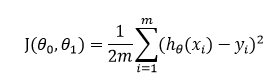
which is the sum of the square of the residual difference.

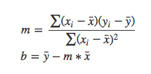
Ordinary Least Squares

It is the estimator technique used to minimize the square of the distance between the predicted values and the actual values. To use the OLS method, we apply the below formula to find the equation:

If you are interested in the derivation behind the OLS formula, refer here.

Now we have seen the equation, let's create a linear regression model using RM as the independent variable and price as the dependent variable.

def ols(x,y):
    x_mean = x.mean()
    y_mean = y.mean()
    slope = np.multiply((x - x_mean), (y - y_mean)).sum() / np.square((x - x_mean)).sum()
    beta_0 = y_mean - (slope * x_mean)
    
    def lin_model(new_x, slope = slope, intercept=beta_0):
        return (new_x, slope, intercept)

    return lin_model

The OLS function calculates the OLS equation and the lin_model function gives the best fit line for the new dataset.

line_model = ols(X_train, y_train)
new_x, slope, intercept = line_model(X_test)

NOTE: We use training dataset to train and test dataset to test the accuracy.

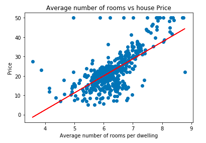
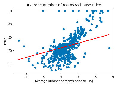
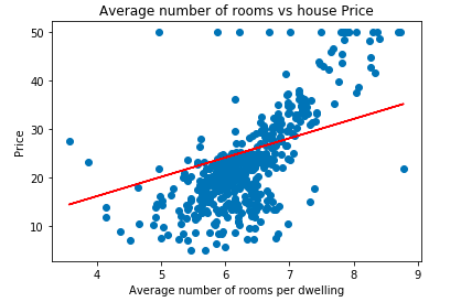
Now that we have the slope and intercept value it's time to plot the best-fit line and visualize the result.

plt.scatter(data['RM'], data['price'])
plt.plot(data['RM'], data['RM'] * slope + intercept, '-r')
plt.xlabel("Average number of rooms per dwelling")
plt.ylabel("Price")
plt.title("Average number of rooms vs house Price")

OUTPUT:

The above code is only for intuitive understanding. In solving industry-based problems, we use the sklearn LinearRegression function to find the best-fit line, which uses an OLS estimator.

y = data['price'].values.reshape(-1, 1)
X = data['RM'].values.reshape(-1, 1)

from sklearn.model_selection import train_test_split
X_train, X_test, y_train, y_test = train_test_split(X, y, test_size = 0.33, random_state = 5)

from sklearn.linear_model import LinearRegression
lm = LinearRegression()
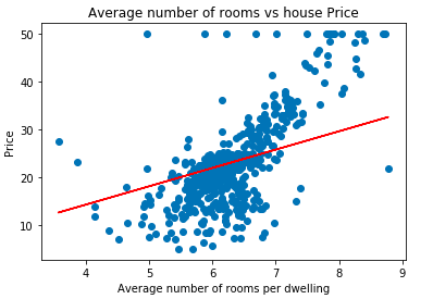
lm.fit(X_train, y_train)

In the code shown above, we created a linear model which fits the scatter plot. Let's see the best-fit line that the model has learned during the training process.

import matplotlib.pyplot as plt

plt.scatter(data['RM'], data['price'])
plt.plot(data['RM'], data['RM'] * lm.coef_[0] + lm.intercept_, '-r')
plt.xlabel("Average number of rooms per dwelling")
plt.ylabel("Price")
plt.title("Average number of rooms vs house Price")

OUTPUT:

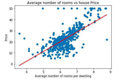
As we can see the plot plotted manually using the OLS function and sklearn LinearRegression function is the same. This is expected as the sklearn Linear Regression function uses an OLS estimator to find the best-fit line.

Mean Square Error or Sum of Squared Residuals

Residual is the measure of the distance from a data point to a regression line. The objective while defining the linear regression line should be minimum residual distance.

The sum of residuals is the square of the difference between the predicted point and the actual point. We need to minimize the Sum of Squared Residuals also known as Mean Square Error (MSE) to obtain the best-fit line.

We have two different approaches to do so:

1. Differential
2. Gradient Descent

Here, we will be discussing Gradient Descent as it is the most industry widely used approach.

Gradient Descent

Gradient Descent is a widely used algorithm in Machine Learning and is not specific to Linear Regression. Gradient descent is widely used to minimize the cost function. 

NOTE: We have used the same cost function to calculate best fit line using OLS estimator.

We differentiate the gradient descent of linear regression with respect to \(\theta_0\) and \(\theta_1\) and we calculate the rate of change of function:

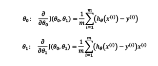
We repeat the steps until convergence.

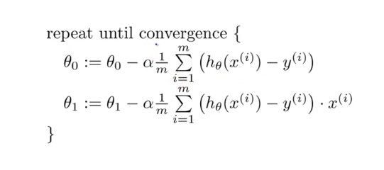
Here α, alpha, is the learning rate, or how quickly we want to move towards the minimum.

NOTE: We should be careful choosing the α. As if we choose α too large we can overshoot the minimum and if α is too small algorithm can take a lot of time to find a minimum of the function.

There are different three types of Gradient Descent Algorithms depending on the dataset:

1. Batch Gradient Descent
2. Stochastic Gradient Descent
3. Mini-Batch Gradient Descent

Let's start with defining and understanding the gradient descent algorithm for Simple Linear Regression.

Batch Gradient Descent

In Batch Gradient Descent, we try to find the minimum of the cost function using the whole dataset. Let's look at the code to find batch Gradient Descent:

def batch_gradient(X, y, m_current=0, c_current=0, iters=500, learning_rate=0.001):
    N = float(len(y))
    gd_df = pd.DataFrame( columns = ['m_current', 'c_current','cost'])
    for i in range(iters):
        y_current = (m_current * X) + c_current
        
        # Cost function J(theta0, theta1)
        cost = sum([data**2 for data in (y_current - y)]) / 2*N
        
        # Diffrential with respect to theta 0 Gradient Descent
        c_gradient = (1/N) * sum(y_current - y)
        
        # Diffrential with respect to theta 1 Gradient Descent
        m_gradient = (1/N) * sum(X * (y_current - y))
        
        # Repeat until convergance
        m_current = m_current - (learning_rate * m_gradient)        
        c_current = c_current - (learning_rate * c_gradient)
        
        gd_df.loc[i] = [m_current[0],c_current[0],cost[0]]
    return(gd_df)

In the algorithm shown above:

1. We first define the best-fit line from which we need to start up with
2. We state the cost function that we need to minimize
3. We differentiate the cost function with respect to m (slope) and c (intercept)
4. We calculate the new slope and intercept based on the learning rate defined
5. Finally, we repeat the process unless and until we find the minimum

cost_gradient = batch_gradient(X,y)

To make sure that Gradient Descent is working as expected we check Gradient Descent after each iteration. And it should decrease after each iteration. The graph shown below represents the Batch Gradient Descent curve:

plt.plot(cost_gradient.index, cost_gradient['cost'])
plt.show()

OUTPUT:

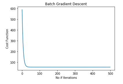
In the graph shown above, as we can see the cost function value has been decreasing, and after one point of iterations, it remains almost constant. This point is our best-fit line. Let's plot the best-fit line:

plt.scatter(data['RM'], data['price'])
plt.plot(data['RM'], data['RM'] * cost_gradient.iloc[cost_gradient.index[-1]].m_current + 
         cost_gradient.iloc[cost_gradient.index[-1]].c_current, '-r')
plt.xlabel("Average number of rooms per dwelling")
plt.ylabel("Price")
plt.title("Average number of rooms vs house Price")

OUTPUT:

Stochastic Gradient Descent

The computational limitation with Batch gradient descent is solved by the Stochastic Gradient Descent. Here, we take different samples as the batch from the data to perform the gradient descent.

Here, since we use random distribution to create the sample the path taken to reach the minimum is noisy.

Since the path is noisy, therefore it takes a large number of iterations to reach the minimum as compared to batch gradient descent. But still, it's less computationally expensive.

def stocashtic_gradient_descent(X, y, m_current=0, c_current=0,learning_rate=0.5,epochs=50):
    N = float(len(y))
    gd_df = pd.DataFrame( columns = ['m_current', 'c_current','cost'])
    
    for i in range(epochs):
        rand_ind = np.random.randint(0,len(y))
        X_i = X[rand_ind,:].reshape(1,X.shape[1])
        y_i = y[rand_ind].reshape(1,1)
        
        y_predicted = (m_current * X_i) + c_current
        cost = sum([data**2 for data in (y_predicted - y_i)]) / 2 * N
        m_gradient = (1/N) * sum(X_i * (y_predicted - y_i))
        c_gradient = (1/N) * sum(y_predicted - y_i)
        m_current = m_current - (learning_rate * m_gradient)        
        c_current = c_current - (learning_rate * c_gradient)
        gd_df.loc[i] = [m_current[0],c_current[0],cost[0]]
    return(gd_df)

In the algorithm shown above the only change with respect to batch gradient descent is LOC where we are selecting a sample from the dataset instead of running gradient descent on the whole of a dataset.

cost_history = stocashtic_gradient_descent(X_train,y_train)

To make sure that Gradient Descent is working as expected we check Gradient Descent after each iteration. The graph shown below represents the Stochastic Gradient Descent curve:

plt.plot(cost_history.index, cost_history['cost'])
plt.xlabel('No if Iterations')
plt.ylabel('Cost Function')
plt.title('Stocashtic Gradient Descent')
plt.show()

OUTPUT:

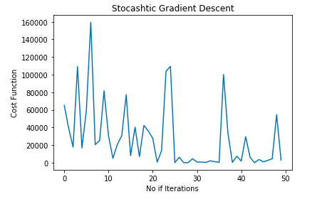
NOTE: As you might have observed the pattern followed by Stochastic Gradient Descent is a bit noisy.

Let's plot the best-fit line using the parameters obtained from Stochastic Gradient Descent:

plt.scatter(data['RM'], data['price'])
plt.plot(data['RM'], data['RM'] * cost_history.iloc[cost_history.index[-1]].m_current 
+ cost_history.iloc[cost_history.index[-1]].c_current, '-r')
plt.xlabel("Average number of rooms per dwelling")
plt.ylabel("Price")
plt.title("Average number of rooms vs house Price")

OUTPUT:

Sklearn SGDRegressor

Sklearn also provides the function SGDRegressor to find the best-fit line using Stochastic Gradient Descent. Refer to the code shown below:

clf = linear_model.SGDRegressor(max_iter=1000, tol=0.001)
clf.fit(X_train, y_train.reshape(len(y_train),))

It will give the optimized coefficients. Let's plot the graph showing the best-fit curve:

plt.scatter(data['RM'], data['price'])
plt.plot(data['RM'], data['RM'] * clf.coef_[0] + clf.intercept_, '-r')
plt.xlabel("Average number of rooms per dwelling")
plt.ylabel("Price")
plt.title("Average number of rooms vs house Price")

OUTPUT:

Mini-Batch Gradient Descent

This is a much more practical approach in the industry. This approach uses random samples but in batches. (i.e. We do not calculate the gradient descent of each sample but for the group of observations leading to much better accuracy)

def minibatch_gradient_descent(X, y, m_current=0, c_current=0,learning_rate=0.1,epochs=200, 
                                                   batch_size =50):
    N = float(len(y))
    gd_df = pd.DataFrame( columns = ['m_current', 'c_current','cost'])
    
    indices = np.random.permutation(len(y))
    X = X[indices]
    y = y[indices]
        
    for i in range(epochs):
        X_i = X[i:i+batch_size]
        y_i = y[i:i+batch_size]
        
        y_predicted = (m_current * X[i:i+batch_size]) + c_current
        cost = sum([data**2 for data in (y_predicted - y[i:i+batch_size])]) / 2 *N
        m_gradient = (1/N) * sum(X_i * (y_predicted - y_i))
        c_gradient = (1/N) * sum(y_predicted - y_i)
        m_current = m_current - (learning_rate * m_gradient)
        c_current = c_current - (learning_rate * c_gradient)
        gd_df.loc[i] = [m_current[0],c_current[0],cost]
    return(gd_df)

In the code shown above, We are shuffling the observations and then creating the batches. Thereafter we are calculating the gradient descent on the batches created.

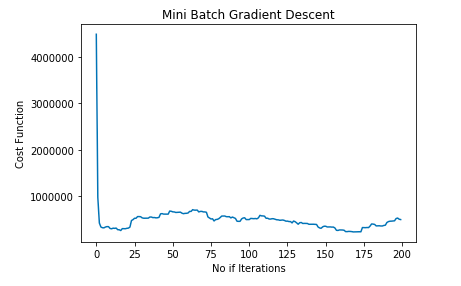
minibatch_cost_history = minibatch_gradient_descent(X_train,y_train)

To make sure that Gradient Descent is working as expected we check Gradient Descent after each iteration. The graph shown below represents the Mini Batch Gradient Descent curve:

plt.plot(minibatch_cost_history.index, minibatch_cost_history['cost'])
plt.xlabel('No if Iterations')
plt.ylabel('Cost Function')
plt.title('Mini Batch Gradient Descent')
plt.show()

OUTPUT:

Let's plot the best-fit line using the parameters obtained from Mini Batch Gradient Descent:

plt.scatter(data['RM'], data['price'])
plt.plot(data['RM'], data['RM'] * minibatch_cost_history.iloc[minibatch_cost_history.index[-1]].m_current + minibatch_cost_history.iloc[minibatch_cost_history.index[-1]].c_current, '-r')
plt.xlabel("Average number of rooms per dwelling")
plt.ylabel("Price")
plt.title("Average number of rooms vs house Price")

OUTPUT:

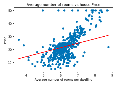
As you might have noticed the result of Batch, Stochastic and MiniBatch are almost the same. (i.e. The best-fit line is almost the same in the three approaches.) It makes sense because we are using the same algorithm with only a difference in computational expense.

Multicollinearity

Before we conclude the post there is one last concept that you should be aware of when training a linear regression model which is about multicollinearity.

Multicollinearity is the occurrence of high intercorrelations among two or more independent variables in a multiple regression model. In simple terms, multicollinearity occurs if there are two independent variables that are correlated to each other. This generally skews the results as the dependent variable can be explained using one of the multicollinear variables.

Two variables are considered perfectly collinear if their correlation coefficient is +/- 1.0. As correlation coefficient which is represented as "r" measures the strength of the linear relationship between two variables.

Correlation shows the relation between two variables. The correlation coefficient shows the measure of correlation. To learn more about correlation, refer to the post Confound between Covariance and Correlation? Me too.

Variance Inflation Factor (VIF)

Apart from correlation we also use VIF to measure the severity of multicollinearity in regression analysis. Variance inflation factor (VIF) is used to detect the severity of multicollinearity in the ordinary least square (OLS) regression analysis.

VIF is calculated as shown below:

$$VIF_i = {1 \over 1 - R^2_i}$$

,where \(R^2_i\) is the unadjusted coefficient of the \(i^{th}\) independent variable on the remaining independent variables. The general rule of thumb for the VIF range is as shown below:

• VIF > 10 is a serious concern and there exists multicollinearity
• VIF > 5 or VIF > 10 is problematic
• VIF < 4 is fine and there doesn't exist multicollinearity

Correction of Multicollinearity

It is essential to detect and correct multicollinearity to build accurate linear regression models. There are two simple and commonly used ways to correct multicollinearity, as listed below:

1. The first one is to remove the highly correlated variables (one by one). As the information provided by the correlated variables is redundant.
    
2. The second method is to use principal components analysis (PCA) or partial least square regression (PLS) instead of OLS regression. PLS regression can reduce the variables to a smaller set with no correlation among them. In PCA, new uncorrelated principal components are created.

BONUS: Akaike Information Criterion (AIC)

The Akaike information criterion (AIC) is a metric that is used to compare the fit of several regression models.

It is calculated as:

$$AIC = 2K – 2ln(L)$$

Where, 

• K: The number of model parameters. The default value of K is 2, so a model with just one predictor or independent variable will have a K value of 2+1 = 3.
• ln(L): The log-likelihood of the model.

The AIC helps to find the model that explains the most variation in the data while penalizing models that use an excessive number of parameters or independent variables. Once we have fit several regression models, we can compare the AIC value of each model. The lower the AIC, the better the model fit.

Summary

We started defining what Linear Regression is and we defined a few metrics like ESS, RSS, TSS, RSE, and R squared that help us to find the best-fit line and evaluate model performance. After deep understanding, we defined the cost function and used various techniques to minimize it:

1. Ordinary Least Square - OLS Estimator
2. Mean Square Error - MSE

that can be used to find the best-fit line. We defined the formula for OLS and wrote a Python function to calculate OLS. Thereafter we defined the MSE function and understood the concept of Gradient Descent that is used to minimize MSE. We saw three different types of gradient descent approaches:

1. Batch Gradient Descent
2. Stochastic Gradient Descent
3. Mini Batch Gradient Descent

While understanding the above concepts we also learned about the sklearn packages LinearRegression and SGDRegressor which use OLS and Stochastic Gradient Descent approaches respectively to find the best fit line.

NOTE: These are not the best models, in fact, these are the bad models with R squared as negative. The above piece of work is only for demonstration purpose. Why I have choosed this if I know these are bad models? To explain about the limitations of the Linear Regression which I will be rolling out shortly.

Do you have any feedback, suggestions, or questions? Let's discuss them in the comment section below.