Limitations of the Linear Regression

In the previous post, we discussed a Simple Linear Regression detailed Explanation. I recommend you to go through the post to have a detailed understanding of the Simple Linear Regression. There are a few assumptions that Linear Regression has to find the best fit line.

NOTE: This assumptions hold true for Simple and Multi Linear Regression.

Let's understand the assumptions of Linear Regression and discuss them in detail.

Limitations of the Linear Regression

We cannot apply linear regression blindly on any of the datasets. The data has to be in the constraint such that we can apply a Linear Regression algorithm on it. There are a few limitations that need to be satisfied. These are:

• Linearity
• Constant Error Variance
• Independent Error Terms or No autocorrelation of the residuals
• Normal Errors
• Multicollinearity
• Exogeneity or Omitted Variable Bias

Linearity

The relationship between the target variable and the independent variable must be linear.

Sometimes the straight line may not be the right fit to data and we may need to choose the polynomial function like under root, square root, log, etc to fit the data. Let's look at an example shown below:

NOTE: Even though we use the nonlinear function but the nature of the curve is still linear as we using the polynomial function to add a new term to the linear function.

Constant Error Variance (Homoscedasticity or no Heteroskedasticity)

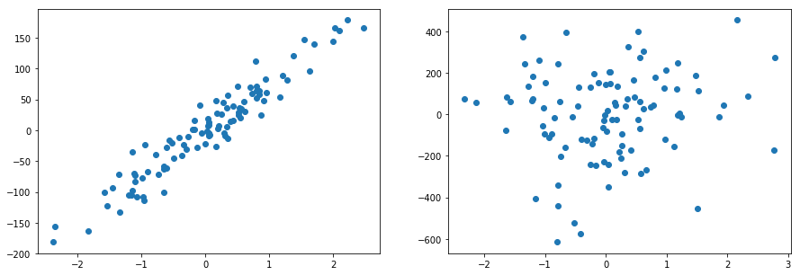
Homoscedasticity describes a situation in which the error term is the same across all values of the independent variables.

If we have a dataset where the spread of the data or variance increases as X increases then there is a problem. And it would not be the best idea to use linear regression in such scenarios.

Or in other words, the residuals of the points should not follow any pattern. Let's plot a scatter plot between dependent and independent variables:

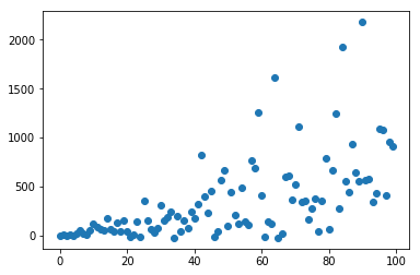
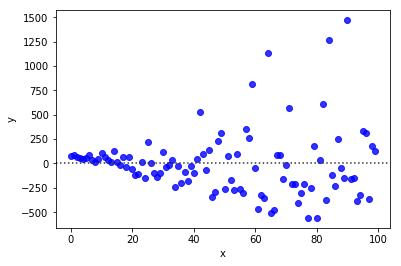
To check the heteroskedasticity of the data, we plot residual plot and the expected result is that the plot should be randomly spread out and there should not be any patterns.

Independent Error Terms or No autocorrelation of the residuals

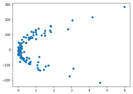
The residual term should not depend on the previous residual term. Or in other words, y(x) is dependent on y(x+1). This assumption makes sense when we are dealing with time series related data.

Consider an example of the stock price, where the current price is dependent on the previous price. This violates the assumption of the Independent Error Terms.

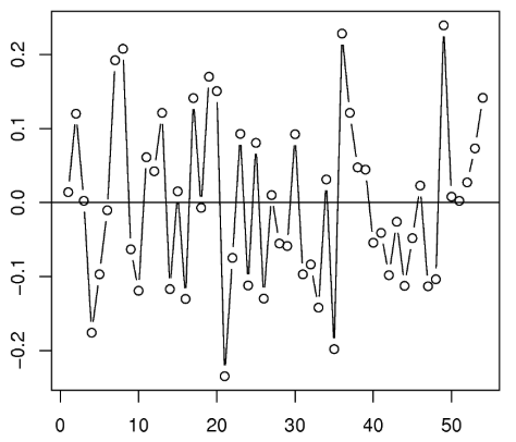
NOTE: In the example shown above we have drawn a residual plot and clearly we can see that residual is dependent on the previous residual.

Normal Errors

Residual should follow a bell-shaped distribution with the mean of 0. In other words, if we draw a histogram of the residual term it should be a bell shape curve having a mean close to 0 with constant standard deviation.

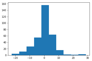
The normality assumption of errors is important because while predicting individual data points, the confidence interval around that prediction assumes that the residuals are normally distributed.

We have to use ‘Generalised Linear Models’ if we want to relax the normality assumptions.

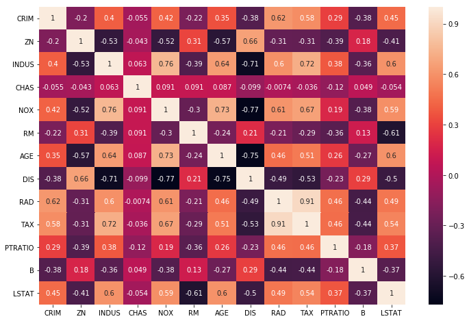
Multicollinearity

Multicollinearity occurs when the independent variable X depends on the other independent variable. 

In a model with correlated variables, it is difficult to figure out the true relationship between the independent and dependent variable. In other words, it becomes difficult to find out which independent variable is actually contributing to predict the dependent variables.

Additionally, with correlated variables, the coefficient of the independent variable depends on the other variables present in the dataset. If this happens we will end up with an incorrect conclusion of independent variables contributing to the prediction of the dependent variable.

The best way to check for the multicollinearity is by plotting heatmap. The variables having high correlations are multicollinearity.

NOTE: As of now we are just dealing with the model having a single independent variable. This will make sense when we move to the linear regression model with multiple independent variables.

Exogeneity or Omitted Variable Bias

Before we understand Exogeneity it's important to know when we generate a linear regression line there is an error associated with it. (It is different from residual).

y = ax1 + bx2 + . . . . . + nxn +

where  represents all of the factors that impact the target variables and is not included in the model.

Consider a feature A which is not included in the model. So it's the part of the error term. And also A has a high correlation with the x2 and y variable. This will make coefficient b as biased and will not be a true coefficient. (i.e. Sample is not a reflection of population value)

Or in other words, A variable is correlated with both an independent variable in the model, and with the error term. And the true model to be estimated is:

but we omit zi when we run our regression. Therefore, zi will get absorbed by the error term and we will actually estimate:

      (where )

If the correlation of  and  is not 0 and  separately affects , then  is correlated with the error term .

Therefore Exogeneity or Omitted Variable Bias occurs when a statistical model leaves out one or more relevant variables.

The best way to deal with endogeneity concerns is through instrumental variables (IV) techniques. And the most common IV estimator is Two Stage Least Squares. (TSLS)

Summary

In this post, we discussed the limitations of the Linear Regression. We did a detailed analysis to understand each of the limitations and how to detect them in the model.

Please let me know your views in the comment section below.