Lasso and Ridge Regression Detailed Explanation

In Linear Regression we saw that the complexity of the model is not controlled. Linear Regression only tries to minimize the error (e.g. MSE) and may result in arbitrarily complex coefficients.

The model which we are developing should be as simple as possible but not simpler.

Regularization is a process used to create an optimally complex model, i.e. a model which is as simple as possible while performing well on the training data. 

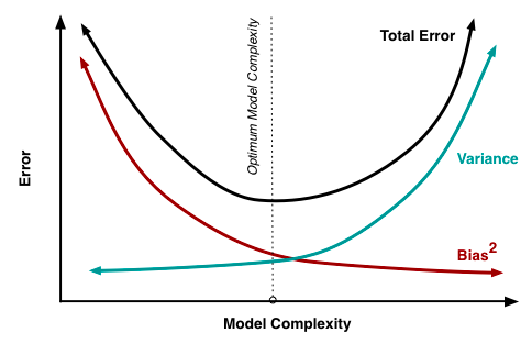
As we can see from the diagram shown above our model should not be very complex and at the same time, it should not be very naive.

Therefore we have regularized regression which is an improvement to Linear Regression and monitors the complexity of the model. The two most common regularization techniques are:

• Ridge Regression
• Lasso Regression

The Lasso and Ridge regressions are examples of constrained minimization problems. 

Also, note that unlike linear regression where the objective is to minimize error term, the objective of regularized regression has two parts i.e. Error Term and Regularized Term. 

Let's define the most common regularization techniques Ridge and Lasso Regression.

Ridge Regression

Ridge regression (L2 regularization) is where we add the sum of the square of coefficients to the error term. This will help to control the complexity of the model as:

• If we want to minimize the cost function then the coefficients need to be small. Doing this will maintain the model complexity.
• On the other hand, if our coefficients are large and complex, then the cost function will be penalized. Therefore adding the constraint to the algorithm as the model is penalized if coefficients are large.

The objective function also known as cost function for ridge regression is given by:

$$cost(w) = \sum_{i = 1}^n(y_i - w^Tx_i)^2 + \sum_{i = 1}^k \lambda w_i^2$$

where,

• \(w_i^2\) (Sum of square of coefficients) is the regularization term controlled by the regularization coefficent  \(\lambda \). 
• \(\sum_{i = 1}^n(y_i - w^Tx_i)^2 \) is the error term.
• \(\lambda\) is the tunning parameter that decides the level we want to penalize the flexibility of the model.

Here the objective is to not only minimize the error term but also we need to minimize regularization term added. Therefore it will help to control the higher coefficients of the model.

Matrix Representation:

$$\bar \alpha = (X^TX + \lambda I)^{-1}X^Ty_i$$

NOTE: In Linear Regession where soltion is given by \(\bar \alpha = (X^TX)^{-1}X^Ty_i\), we cannot gurantee that X matrix is invertable or in other words that inverse of matrix exists. But here in case Ridge Regularization the \((X^TX + \lambda I)\) is far more likely to be invertable. (i.e. Determinant of the matrix is non zero)

We use gradient descent similar to the linear regression to find optimal minimum solution:

$$\frac{\partial}{\partial w_j}cost(w) = -2 \sum_{i = 1}^nx_i\{y_i- w^Tx_i\} + 2\lambda w_j$$

We repeat the above step unless we reach the optimal solution:

$$= w^t_j - \eta[-2 \sum_{i = 1}^nx_i\{y_i- w^Tx_i\} + 2\lambda w_j]$$

Lasso Regression

Lasso regression (L1 Regularization also known as Least Absolute Shrinkage and Selection Operator) is another variation which is different from the Ridge Regression only in terms of penalizing the higher coefficients.

The cost function for lasso regression is given by:

$$cost(w) = \sum_{i = 1}^n(y_i - w^Tx_i)^2 + \sum_{i = 1}^k \lambda |w_i|$$

where,

• w are the weights of the model and \(\lambda \) is regularization coefficient or regularisation hyperparameter.
• \(|w_i|\) (sum of absolute values) is the regularization term controlled by the regularization coefficent  \(\lambda \). 
• \(\sum_{i = 1}^n(y_i - w^Tx_i)^2 \) is the error term.

As we were able to converge the cost function of Ridge regression using gradient descent, the same is not possible with lasso regression. The reason is regularization term added here is not differentiable at x=0.

Therefore we use a different technique called coordinate descent to find an optimal solution.

With lasso regression, we end up getting a sparse solution where some of the model parameters or coefficients will be zero. And the objective is to find theta for which the objective function is minimum.

$$\theta^* = argmin[E(\theta)  + \lambda R(\theta)]$$

where \(E(\theta)\) represents the error function and \(\lambda R(\theta)\) represent the regularization term.

Experimental observation is \(\\sparsity(\theta^*)\) (Number of parameters in \(\theta^*\) that are exactly equal to zero.) increases with increase in \(\lambda\).

Comparison of Ridge and Lasso Regression

1. Ridge regression almost always has a matrix representation for the solution while Lasso requires iterations to get to the final solution. So Lasso regressions are computationally more intensive.

2. One of the most important benefits of Lasso regression is that it results in model parameters such that the lesser important features coefficients become zero. In other words, Lasso regression indirectly performs feature selection.

3. Ridge regression is better in the case of the correlated features as compared to Lasso. Because using Ridge all of the features are included in the model but the coefficients will be distributed among them depending on the correlation.

Why Lasso gives a Sparse solution?

Are you still wondering how Lasso Regression helps us in feature selection? Before proceeding and understanding how Lasso Regression gives sparse solutions it's important to understand:

1. The contour of the function
2. Trade-off Between Error and Regularised Term

The contour of the function

Since every point on the plane has a function value associated with it, therefore contours are the join of all the points where the function value is the same.

A contour of a function f(α) is a trace (locus) of the points that satisfy the equation f(α)=c for some constant c.

There are few interesting properties of the contours:

1. No two contours can intersect: A function can't have two different values for a combination of x and y. (In two-dimensional space)
2. Two contours can meet tangentially.

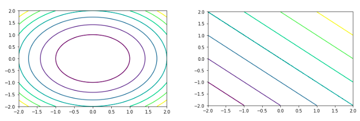
Refer to the example shown below demonstrating the contour plot of the circle and the line:

import matplotlib.pyplot as plt

def Circle(x,y):
    return (x*x+y*y)

def Line(x,y):
    return (x+y)

xx = np.linspace(-2,2,400)
yy = np.linspace(-2,2,400)
[X,Y] = np.meshgrid(xx,yy)

Z_circle = Circle(X,Y)
Z_line = Line(X,Y)

plt.contour(X,Y, Z_circle)
plt.show()

plt.contour(X,Y, Z_line)
plt.show()

Output:

Trade-off Between Error and Regularised Term

We have already seen that the error term with a regularised term is given as:

$$\theta^* = E(\theta)  + \lambda R(\theta)$$

When we increase the value of λ, the error term will increase and the regularisation term will decrease and the opposite will happen when we decrease the value of λ. Proof of this staement is:

Consider a scenario where we have \(\lambda_1\) and  \(\lambda_2\) and the optimal cost function is at value \(\theta_1\) and \(\theta_2\) respectively. Therefore,

$$E(\theta_1) + \lambda_1 R(\theta_1) \le E(\theta_2) + \lambda_1 R(\theta_2)$$

$$E(\theta_2) + \lambda_2 R(\theta_2) \le E(\theta_1) + \lambda_2 R(\theta_1)$$

On rearranging above two equation we get:

$$\lambda_2(R(\theta_2) - R(\theta_1)) \le E(\theta_1) - E(\theta_2) \le \lambda_1(R(\theta_2) - R(\theta_1))$$

As we know \(\lambda_1\)  is greater then \(\lambda_2\) which implies \(\lambda_1 \gt \lambda_2 \), \(E(\theta_1) \ge E(\theta_2) \) and \(R(\theta_1) \le R(\theta_2) \).

The last point to think about is when we are finding the optimal value of theta for which we want to reduce the cost and regularization function. The value of theta should be one where the cost function and regularization function are tangential to each other.

The reason for this being is if the two functions are intersecting for the value of theta. Then keeping one of the values fixed either regularization or cost function we can find another minimum value for the opposite function.

Feature Selection using Lasso Regression

Before understanding why lasso helps in feature selections. Let's see why Ridge regression doesn't produce a sparse solution. Refer to the diagram sown below:

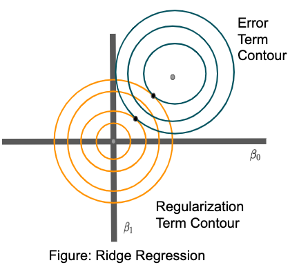
In the diagram shown above, orange contour represents the regularization term contour and blue contour represents the error term contour. And the points where error term and regularization terms are tangential to one another are the possible optimal solutions for which cost function can be minimized.

The chances that the two contours will be tangential to one another on the x or y-axis are very unlikely to happen. Hence it's difficult to have a sparse solution.

But in the case of lasso regularization, there are high chances that the two contours are tangential to one another on x or y-axis. Refer to the diagram shown below:

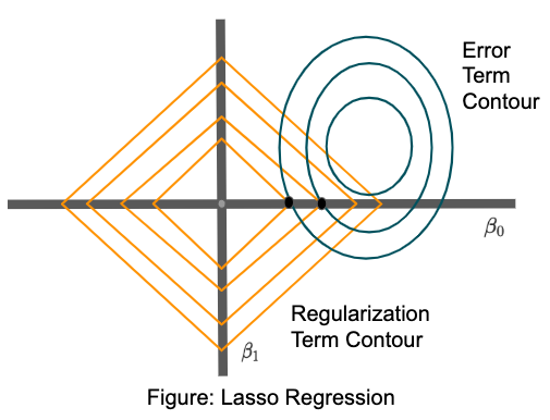
Therefore lasso generates a sparse solution as coefficients for features will be zero. The geometrical proof of why error contour intersects on the axis is beyond the scope of this post.

Summary

In this post, we understand we need Regularized Regression to control the complexity of the model. We saw two regularized techniques:

1. Lasso Regularization
2. Ridge Regularization

We learned how the lambda (a hyperparameter for regularized regression) helps to control the model complexity. We understand Lasso and Ridge Regression in detail and learned why Lasso Regularization results in a sparse solution.