In-depth understanding of Neural Networks and its working

Today using neural network architectures, we can achieve complex tasks like object recognition in images, automatic speech recognition (ASR), machine translation, image captioning, video classification, and a lot more that are challenging for machines to perform. It can do complex tasks using neural networks because artificial neural networks are the most powerful learning models in the field of machine learning.

Neural networks can achieve arguably every task that the human brain can perform. Sounds like a promising revolution in the field of Data Science. Right?

For the post, there are a few prerequisites that are expected you to know. It is expected that you have a basic understanding of statistical concepts, calculus, and matrix multiplication. In this post, we will understand thoroughly how such an architecture of neural networks works. We will also understand the mathematics involved in every stage of training such architecture of neural networks. This is going to be a lengthy article, therefore I recommend you to:

• Bookmark the page and read it in your free time
• Follow 3 iteration process to understand the details of the article

Let's get started.

The Popularity of Neural Network

Before we start understanding how the network works. Let's first answer the question, Why Neural network techniques have been popularized so lately?

There are two fundamental requirements for neural networks to work. These are:

1. Neural networks need the availability of abundant training data.
2. Neural networks require tremendous computational power

Though architecture was available way earlier because of the above two limitations, neural networks have not got the popularity that it deserves. But in the 21st century, because of the high-end machines and the tremendous amount of data availability, neural networks have gained popularity.

The Similarity of Neural Networks with the Human Brain

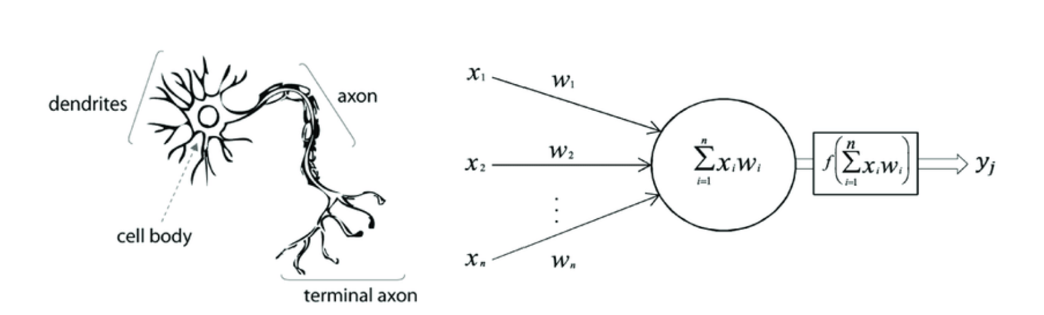
Neural networks have been inspired by the structure of the human brain and its working.

Comparing the human brain with neural networks we can conclude that:

• Our human brain has millions of neurons that keep on learning data fed into it in the form of images, sound, text, etc.
  Artificial Neural Networks are a collection of a large number of simple devices called artificial neurons.
   
• Human Neuron receives signals through their dendrites which are either amplified or inhibited as they pass through the axons to the dendrites of other neurons. Similarly, the neural network learns to inhibit or amplify the input to perform a certain task, such as recognizing a cat, speaking a word, identifying a tree, etc. 

Having a basic understanding of the neurons, let's study the perceptron which is the fundamental building block of artificial neural networks. 

Perceptron

Before we go understand how perceptrons work. I have one question for you. Suppose you want to plan a family trip, from the below factors which are the critical factors for you?

• Trip Expenditure
• Trip Duration
• Hotel Comfort
• Mode of Travelling

How our human brain works is it assigns weight to each of the factors. For me, Trip Duration is the most important factor.

What is the most important factor for you? Let me know your answers in the comment section.

The perceptron works similarly. It takes input signals as inputs and performs a set of simple calculations to arrive at a decision.

Consider a sample perceptron shown below:

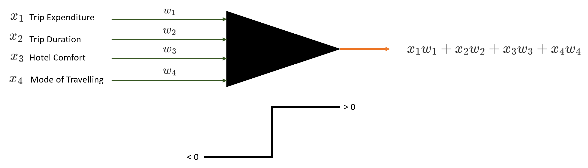
Perceptron takes a weighted sum of multiple inputs (along with a bias) as the cumulative input and applies a step function on the cumulative input. In other words, the perceptron fires (returns 1) if the cumulative input is positive and stays dormant (returns 0) if the input is negative.

The vector notation of the cumulative input is defined as:

$$\text{Cumulative Input} = w^T.x + b = w_1x_1 + w_2x_2 + . . . . . . . + w_kx_k + b$$

Perceptrons can be used in classification tasks as well, where we fit a divider such that it divides the data points into regions.

$$y(w^Tx + b) > 0$$

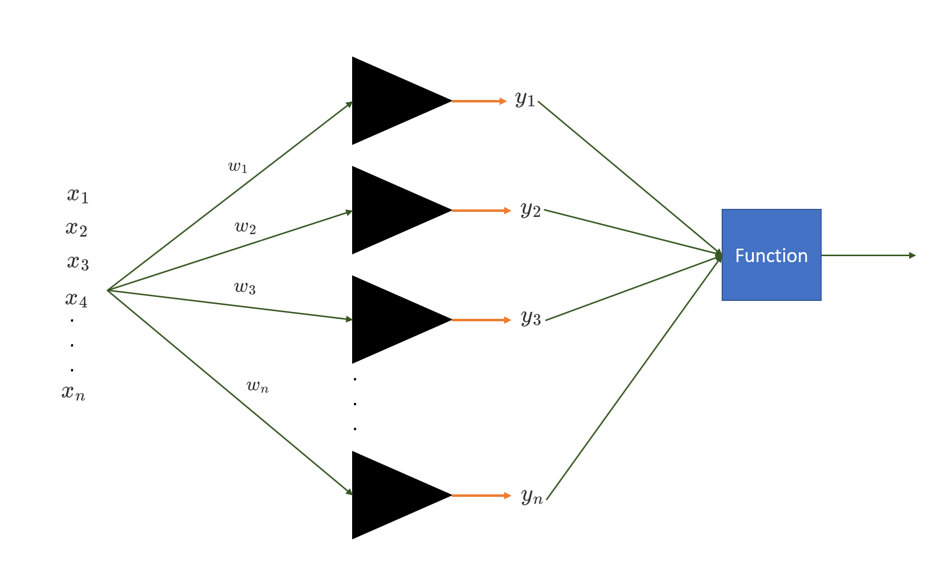
Perceptron can also perform multiclass classification as well. We can use multiple perceptrons where each perceptron classifies data points in a class or another class. Refer to the diagram shown below:

NOTE: We use homogeneous coordinates to represent the perceptron more concisely, where x is represented as  \([x_1, x_2, . . . . , x_d, 1]\)  instead of  \([x_1, x_2, . . . . , x_d]\) and w is represented as \([w_1, w_2, . . . . , w_d, b]\) instead of \([w_1, w_2, . . . . , w_d]\).

Now we know fundamentally what perceptron is, let's look at the iterative solution suggested by Rosenblatt for training the perceptron. 

Training of Perceptron

Rosenblatt suggested an elegant iterative solution to train the perceptron (i.e. to learn the weights involved in the network). He proposed that we start with random weight and keep on adding the error term to the weight till the time we didn't find the valid separator. The error term is the misclassified point from the previous separator.

$$w_{t+1} \Leftarrow w_t + y_{it}.x_{it}$$

where \(x_{it}\) is the misclassified data point in iteration t and \(y_{it}\) is the actual label.

Working of Neurons

Having an understanding of how perceptrons work, let's finally get into the details of Artificial Neural Networks (ANNs). Let us understand the neurons that are used to build ANN networks. Neural networks are a collection of artificial neurons arranged in a particular structure.

The neuron is very similar to a perceptron, the only difference being that there is an activation function applied to the weighted sum of inputs. In perceptrons, the activation function is the step function, though, in artificial neural networks, it can be any non-linear function.

There are six main things needed to define a neural network completely. These are:

1. Network Topology
2. Input Layer
3. Output Layer
4. Activation functions
5. Weights and Biases

Network Topology

Let us start by defining the network topology of neural networks.

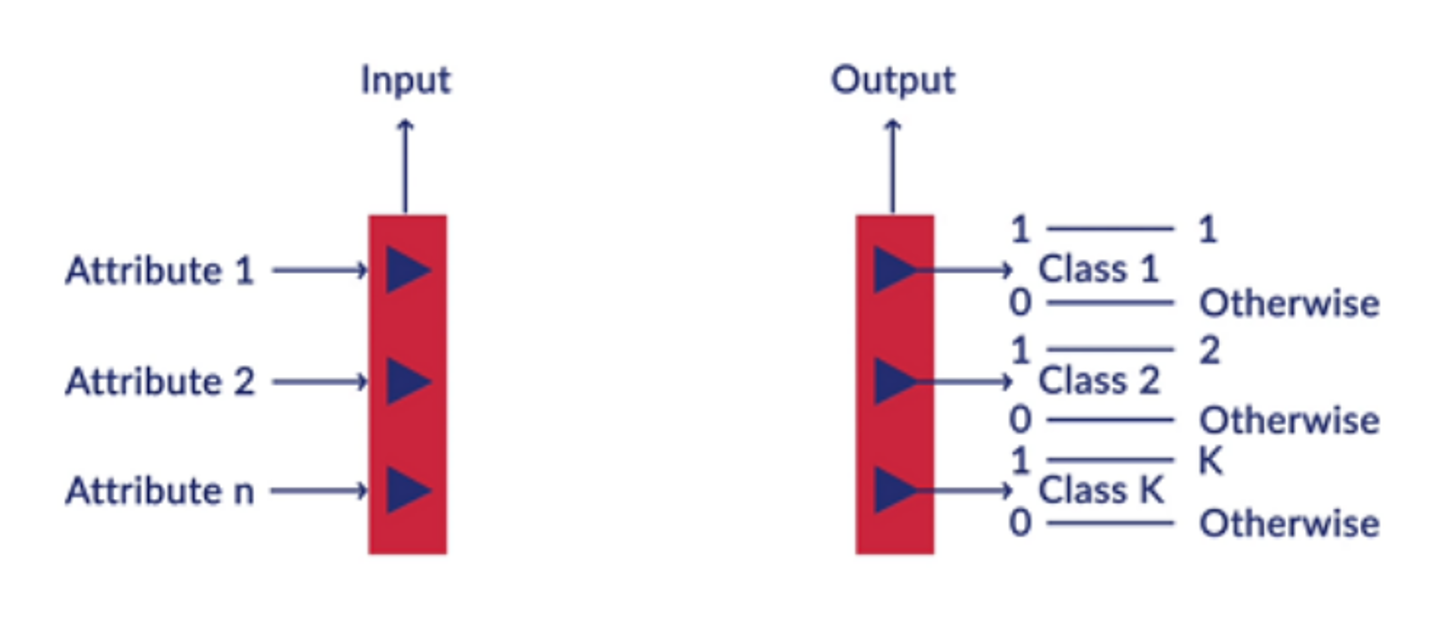
Neurons in a neural network are arranged in layers. The first and the last layer are called the input and output layers. Input layers have as many neurons as the number of attributes in the data set and the output layer has neurons based on the tasks:

• Classification problem: The number of neurons is equal to the number of classes of the target variable.
• Regression problem: The number of neurons in the output layer would be a single numeric variable.

Optionally, there are intermediate layers as well, where weights and bias are the hyperparameters.

Input Layer

The input to the network can only be numeric. So how to solve the problem where the input that we have is text (NLP problems) or Images (Computer Vision problems)?

• Text Data as Input: In the case of text data, we either use a one-hot vector or word embeddings corresponding to a certain word. If our vocabulary size is huge we generally prefer word embeddings over one-hot vectors.
   
• Images as Input: In the case of images (or videos), it's straightforward since images are naturally represented as pixels (arrays of numbers). Where each pixel of the input image is a feature. If we have a grayscale image of size 18 x 18. Our input layer needs 324 neurons. If the image is colored we need 18 x 18 x 3 neurons in the input layer, as the color image has three channels (Red, Green, and Blue).

Output Layer

In the case of a multiclass classification problem, we use the softmax output function at the output layer. The softmax function is represented as:

$$p_i = {e^{w_i.x^{'}} \over \sum_{t=0}^{c-1} e^{w_i.x^{'}}}$$

where c is the number of neurons in the output layer and \(x^{'}\) is the input coming from the previous layer of the network. The \(p_i\) is often called normalizing the vector p.

In the case of binary classification, we use the Sigmoid function at the output layer. We know that for the binary classification, there is only one neuron at the output layer. Therefore:

$$p_0 + p_1 = 1$$

Hence we need to compute either \(p_0\) or \(p_1\). The sigmoid function is just a special case of the softmax function. Therefore \(p_1\) can be represented as:

$$p_1 = {1 \over 1+ e^{(w_0 - w_1).x{'}}} = {1 \over 1+ e^{(w).x{'}}}$$

NOTE: We can drive the above expression from the softmax function which we have defined.

Activation Functions

We know that the weighted sum of neurons passes through the activation function before it goes as an input to the neuron in the next layer. The activation function could be any function, though it should have some important properties such as:

• Activation functions should be smooth i.e. they should have no abrupt changes when plotted. Because decision-making doesn't change abruptly based on any factor.
• The activation function should add nonlinearity. This is done to make complex decisions that are non-nature.

A few popular activation functions used are:

• Logistic function
• Hyperbolic tangent function
• Rectilinear Unit (ReLU)

Properties and Assumptions of Neural Networks

A few properties of Neural Networks are:

1. Neurons in a neural network are arranged in layers where the first and the last layers are called the input and output layers.
2. Input layers have as many neurons as the number of attributes in the data set.
3. The output layer has as many neurons as the number of classes of the target variable in the case of the classification problem.
4. The output layer has one neuron in case of the regression problem.

Commonly industry-used neural networks follow the below assumptions:

1. Neurons are arranged in layers and the layers are arranged sequentially.
2. Neurons within the same layer do not interact with each other.
3. All the inputs enter the network through the input layer and all the outputs go out of the network through the output layer.
4. Neurons in consecutive layers are densely connected, i.e. all neurons in layer l are connected to all neurons in layer l + 1.
5. Every interconnection in the neural network has a weight associated with it, and every neuron has a bias associated with it.
6. All neurons in a particular layer use the same activation function.

Now comes the core part that will help you to understand how exactly the neural network training process works. Having an in-depth understanding of the maths behind neural networks will help you design better neural networks.

Training of the Neural Network

The weight and bias of every neuron need to be trained to get the right predictions. Training of neural networks is similar to any other Machine Learning algorithm like SVM, Linear Regression, etc where the objective is to find optimal weights and biases to minimize the loss function. This optimization is done using the gradient descent algorithm.

Sounds simple? Wait we have an issue here. The loss function that we need to minimize is complex. Let's understand this with the help of an example.

Consider a network where we have 100 neurons in the input and output layers. We have 5 intermediate layers having 100 neurons each.

Now every intermediate layer will have 100 * 100 = 10,000 interconnections for the weight matrics. And we have a 6-layer network (intermediate layer + output layer). So we will be having 10,000 * 6 = 60,000 weights in the entire network.

And we will be having 100 biases for each layer (1 per neuron). And 6 * 100 = 600 in the entire network.

The number of the parameters that we need to minimize is 60,000 + 600 = 60,600 

In simple terms, we are trying to minimize the loss function which has 60,600 parameters. With this, we can imagine how complex the loss function would be.

Note that this is a very simple network while solving actual problems there will be billions of weights and biases that need to be minimized.

Because of the above-defined complexity, there is a two-way propagation that happens in neural networks to optimize the loss function. This includes feedforward and backpropagation as defined below:

• Feedforward: The information flows (or training of the network) in a neural network from the input layer to the output layer. The information flow in this direction is often called feedforward.
   
• Backpropagation: The adjustment of the weights happens at this stage to minimize the loss function. The information flows from the output layer to the input layer which is why it is called backpropagation.

Let's understand them in detail.

Feedforward Neural Networks

Consider an example neural network with two layers (the input layer is not counted). There are three neurons in the input layer, four neurons in the intermediate layer, and one in the output layer. And all neurons are densely connected. Refer to the diagram shown below.

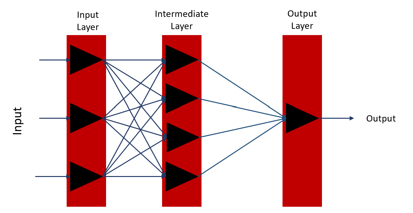
The assumption is that we are starting with some random weight and biases. Let's see the first feedforward propagation from the input layer to the intermediate layer.

Let's consider a single point. Our input vector \(x_i\) is represented as:

$$x_i = [\begin{matrix} x_1 \\ x_2  \\ x_3  \end{matrix}]$$

where the dimension is (3,1)

The output from the intermediate layers is represented as:

$$h^1 = [\begin{matrix} h^1_1 \\ h^1_2  \\ h^1_3 \\ h^1_4  \end{matrix}]$$

And weight matrix is represented as:

$$W^1 = [\begin{matrix} w^1_{11} && w^1_{12} && w^1_{13}\\ w^1_{21} && w^1_{22} && w^1_{23}  \\ w^1_{31} && w^1_{32} && w^1_{33} \\ w^1_{41} && w^1_{42} && w^1_{43}  \end{matrix}]$$

As we know the output from neurons is the activation function of the weighted sum and the bias added. Therefore the output of the intermediate layer is represented as:

$$h^1 = [\begin{matrix} h^1_1 \\ h^1_2  \\ h^1_3 \\ h^1_4  \end{matrix}] =\sigma(W^1.x_i + b) = [\begin{matrix} \sigma(w^1_{11} + w^1_{12} + w^1_{13} + b_1^1) \\ \sigma(w^1_{21} + w^1_{22} + w^1_{23} + b^1_2)  \\ \sigma(w^1_{31} + w^1_{32} + w^1_{33} + b^1_3) \\ \sigma(w^1_{41} + w^1_{42} + w^1_{43} + b^1_4)  \end{matrix}]$$

This completes the forward propagation of a single data point through one layer of the network.

To summarize the steps that we have followed to compute the output of the \(i^{th}\) neuron in the layer l are:

1. Multiply the \(i^{th}\) row of the weight matrix with the output of layer l-1 to get the weighted sum of inputs.
2. Convert the weighted sum to the cumulative sum by adding the \(i^{th}\) bias term of the bias vector.
3. Apply the activation function, σ(x) to the cumulative input to get the output of the \(i^{th}\) neuron in layer l.

Having an understanding of how a feedforward network works. Let's write a pseudo code for it. 

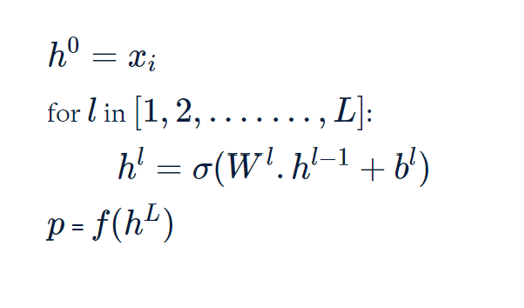
• We started with the input layer as the \(i^{th}\) data point
• We calculated the output from the intermediate layers
• For the output layer, we use different activation functions based on the problem statement as discussed above in the activation function section.

Feedforward for n data points

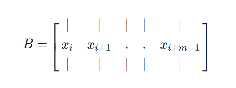
So far we have written a pseudo code to perform feedforward for a single data point. Now let's look at how we can perform feedforward for n data points.

Writing a for loop to perform feedforward is not a good idea because of computational reasons. Therefore we use vectorized computation techniques.

Vectorized implementation means performing the computation for multiple data points using matrices. 

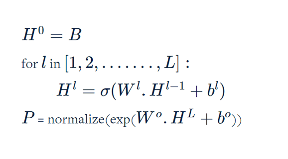
As you might have observed there are only notation changes and the algorithm remains the same as the feedforward of the single data point. And not instead of passing a single data point we now pass a matrix to the input layer.

As we see we can do feedforward using the product of matrices and vectors allowing the neural network an opportunity to do the parallelized computation and use GPUs.

We are set up to do the backward propagation now. Let's see how the backpropagation happens from the output layer towards the left.

Backpropagation in Neural Networks

Once we are done with the feedforward, we need to calculate the loss function. The loss function will define the state we are at. Let's define the loss function before proceeding further.

$$G(w,b) = {1 \over n}\sum^n_{i=1}L(F(x_i), y_i)$$

The loss function is defined as the \(F(x_i)\) (which depends on the weight and biases) and actual output \(y_i\). The average loss function across all data points is represented as \(G(w,b)\).

NOTE: A commonly used loss function for classification problems is the cross-entropy loss.

Let us consider a problem statement where we have two input features and three output classes in the defined neural network. Refer to the diagram shown below.

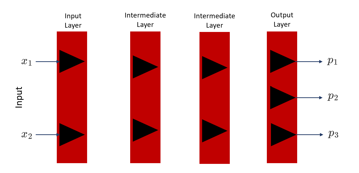
Since our problem is a multiclass classification problem, therefore our loss function will be a cross-entropy loss function.

$$L= -(y_1 log(p_1) + y_2 log(p_2) + y_3 log(p_3))$$

where y are the actual outputs and p are the predicted outputs. And our objective is to find \(\frac{\partial L}{\partial W}\) and \(\frac{\partial L}{\partial b}\).

We also define a notation to represent the weighted sum of inputs for simplifying the calculations as below:

$$z^l = W^l.h^{l-1} + b^l$$

Now, let's consider the last layer (output layer) and find the gradient \(\frac{\partial L}{\partial W^3}\). The issue with calculating the gradient is that function L is not directly dependent on W.

If not directly, but indirectly they are related. L is related to p -> p is related to \(z^3\) -> \(z^3\) is related to \(W^3\) -> \(W^3\) with \(h^2\), and so on. We will use this observation to drive the expressions.

Expression showing p is related to \(z^3\)

$$p_i = {e^{z_i} \over  e^{z_1} + e^{z_2} + e^{z_3}}$$

$$\frac{\partial p_1}{\partial z_1^3} = p_1(1 - p_1)$$

In a similar way

$$\frac{\partial p_2}{\partial z_1^3} = -p_1p_2$$

$$\frac{\partial p_3}{\partial z_1^3} = -p_1p_3$$

Similarly, we can calculate the gradient of p with respect to \(z^3_2\) and \(z^3_3\). With this, we will be having an expression for  \(\frac{\partial q}{\partial z^3}\).

We use the chain rule of differentiation to calculate \(\frac{\partial L}{\partial z^3}\) which is represented as:

$$ \frac{\partial L}{\partial z^3} = - (\frac{\partial (y_1log(p_1))}{\partial p_1}  \frac{\partial p_1}{\partial z^3_1}  + \frac{\partial (y_2log(p_2))}{\partial p_2}  \frac{\partial p_2}{\partial z^3_1} + \frac{\partial (y_3log(p_3))}{\partial p_3}  \frac{\partial p_3}{\partial z^3_1})$$

On substituting the values and solving the equation we get the following expressions:

$$ \frac{\partial L}{\partial z^3_1} = p_1 - y_1$$

$$ \frac{\partial L}{\partial z^3_2} = p_2 - y_2$$

$$ \frac{\partial L}{\partial z^3_3} = p_3 - y_3$$

Therefore the vector notation can be written as:

$$ \frac{\partial L}{\partial z^3} = p - y$$

Expression showing L is related to \(W^3\)

We again use the chain rule of differentiation to calculate \(\frac{\partial L}{\partial w^3}\).

$$ \frac{\partial L}{\partial W^3} = \frac{\partial L}{\partial z^3} \frac{\partial z^3}{\partial W^3}$$

We already know the value of the \(\frac{\partial L}{\partial z^3}\) and we need to find the value of \(\frac{\partial z^3}{\partial W^3}\) to update our first set of weight.

$$z^3 = W^3.h^2 + b^3$$

We use above equation to calculate \(\frac{\partial z^3}{\partial W^3}\).And once calculated we can find \(\frac{\partial L}{\partial w^3}\). The output of the calculation is

$$\frac{\partial L}{\partial w^3} = \frac{\partial L}{\partial z^3}.(h^2)^T$$

Having calculated the expression we can update the first weight in the network.

$$W^3 = W^3 - \alpha \frac{\partial L}{\partial W^3}$$

Updating weights of the previous layer

Similarly, we will be updating the weight of the previous layer \(W^2\), where we calculate \(\frac{\partial L}{\partial w^2}\).

To compute \(\frac{\partial L}{\partial h^2}\), we will use \(\frac{\partial L}{\partial h^2}\) and \(\frac{\partial L}{\partial z^2}\) as the intermediary variables.

To calculate \(\frac{\partial L}{\partial h^2}\) we again use the chain rule of differentiation and intermediary variable \(z^3\)

$$\frac{\partial L}{\partial h^2_1} = \frac{\partial L}{\partial z^3_1}. \frac{\partial z^3_1}{\partial h^2_1} + \frac{\partial L}{\partial z^3_2}. \frac{\partial z^3_2}{\partial h^2_1}$$

$$\frac{\partial L}{\partial h^2_2} = \frac{\partial L}{\partial z^3_1}. \frac{\partial z^3_1}{\partial h^2_2} + \frac{\partial L}{\partial z^3_2}. \frac{\partial z^3_2}{\partial h^2_2}$$

Since we know that,

$$z^3_1 = w^3_{11}h^2_1 + w^3_{12}h^2_2 + b^3_1 $$

$$z^3_2 = w^3_{21}h^2_1 + w^3_{22}h^2_2 + b^3_2 $$

Differentiating above equations with respect to \(h^2_1\) we get \(\frac{\partial z^3_1}{\partial h^2_1}\) as \(W^3_{11}\) and \(\frac{\partial z^3_2}{\partial h^2_1}\) as \(W^3_{21}\). Also differentiating with respect to \(h^2_2\) we get \(\frac{\partial z^3_1}{\partial h^2_2}\) as \(W^3_{12}\) and \(\frac{\partial z^3_2}{\partial h^2_2}\) as \(W^3_{22}\).

On plugging in the value we get

$$\frac{\partial L}{\partial h^2_1} = \frac{\partial L}{\partial z^3_1}. w^3_{11} +  \frac{\partial L}{\partial z^3_2}. w^3_{21}$$

$$\frac{\partial L}{\partial h^2_2} = \frac{\partial L}{\partial z^3_1}. w^3_{12} +  \frac{\partial L}{\partial z^3_2}. w^3_{22}$$

which can be generalized as

$$\frac{\partial L}{\partial h^l}  = (w^{l+1})^T.\frac{\partial L}{\partial z^{l+1}}$$

Now after calculating \(\frac{\partial L}{\partial h^2}\) next step is to calculate \(\frac{\partial L}{\partial z^2}\). To compute \(\frac{\partial L}{\partial z^2}\) we use the chain rule of differentiation and intermediary variable \(h^2\) which is represented as:

$$h^2 = [\begin{matrix} h_1^2 \\ h_2^2 \end{matrix}] = [\begin{matrix} \sigma(z_1^2) \\ \sigma(z_2^2) \end{matrix}]$$

Therefore \(\frac{\partial L}{\partial z^2}\) is represented as

$$\frac{\partial L}{\partial z^2_1} = \frac{\partial L}{\partial h^2_1}.\frac{\partial h^2_1}{\partial z^2_1} + \frac{\partial L}{\partial h^2_2}.\frac{\partial h^2_2}{\partial z^2_1} = \frac{\partial L}{\partial h^2_1}. \sigma{'}(z^2_1)$$

$$\text{Since } \frac{\partial h^2_1}{\partial z^2_1} = \sigma{'}(z^2_1) \text{ and } \frac{\partial h^2_2}{\partial z^2_1} = 0$$

$$\text{And in same way } \frac{\partial L}{\partial z^2_2} = \frac{\partial L}{\partial h^2_2}.\sigma{'}(z^2_2)$$

which can be generalized as

$$\frac{\partial L}{\partial z^l} = \frac{\partial L}{\partial h^l}*\sigma{'}(z^l)$$

NOTE: Here product is the element wise product and it's not dot product.

Having calculated \(\frac{\partial L}{\partial h^2}\) and \(\frac{\partial L}{\partial z^2}\) now its an easy task to calculate  \(\frac{\partial L}{\partial W^2}\). We have already calculated \(\frac{\partial L}{\partial w^3}\)

$$\frac{\partial L}{\partial w^3} = \frac{\partial L}{\partial z^3}.(h^2)^T$$

Therefore by symmetry, we can calculate,

$$\frac{\partial L}{\partial w^2} = \frac{\partial L}{\partial z^2}.(h^1)^T$$

which can be generalized as

$$\frac{\partial L}{\partial w^l} = \frac{\partial L}{\partial z^l}.(h^{l-1})^T$$

Now having the weight loss gradient calculated we can simply calculate the new weights as

$$W^l = W^l - \alpha \frac{\partial L}{\partial W^l}$$

With this, we complete the backward propagation as well. Hectic isn't it? I suggest reiterating and going slow if this is overwhelming for you.

So far we have done a feedforward and backward propagation for the single data point. In a real-time scenario, it will be computationally expensive to iterate for single data points. To avoid this we train neural networks in batches.

Batch Training of Neural Networks

We have briefly covered the training of neural networks in batches in the feedforward section of the article. Let's discuss now how we use the concept to do end-to-end training of neural networks in batches.

We use the Stochastic Gradient Descent (SGD) technique to train the neural network in batches. And we take an average gradient of each batch to update the weights.

Using this technique there is a risk of ineffective training as we are updating the weights based on the small batch and not an entire dataset. To avoid this we use epoch, where for each epoch we reshuffle all the data points, divide the reshuffled set into batches, and update weights based on the gradient of each batch. 

Summarization of batch training of Neural Networks using SGD:

• We specify the number of epochs (like 10, 20, 50, 100, etc.) for training NN.
• We specify the number of batches (like 32, 64, 128, etc.)
• At the start of each epoch, the data set is reshuffled and divided into batches.
• The average gradient of each batch is then used to make a weight update.
• The same process is repeated for every epoch.

Most libraries such as TensorFlow, and Keras also follow the above-stated approach to training neural networks.

There are advantages that we get when training neural networks with the SGD approach:

• Faster Computational performance
• Reach global minima instead of getting stuck at local minima: Since we start with a different point in each epoch, therefore, an algorithm is exploring different options.

Overfitting

We have seen that the neural network is a complex model and there are a lot of parameters that need to be trained. Therefore there are high chances that the model overfits.

Regularization

To avoid the complexity of the model we use regularization as we do for any other machine learning model. If you are not sure about regularization, please refer to the post, Lasso and Ridge Regression Detailed Explanation.

We apply L1 or L2 regularization in the case of neural networks as well.

NOTE: We only normalize the weights since it has been empirecally proved that normalizing bias has a negative impact on the performance.

Dropouts

Apart from the L1 and L2 normalization techniques we also use dropouts to control the model complexity.

Dropouts are another popular regularization technique that is used to control overfitting. To control overfitting, we randomly drop out a few connections within the layer. Therefore, Dropout is implemented per layer in a neural network. Let's see how we can train a network layer to drop out connections.

The dropout operation is performed by multiplying the weight matrix with the mask vector. Consider a 3 x 3 weight matrix, now the shape of the alpha vector should be 3 x 1 to carry out the multiplication.

We also need to specify the probability of connection that we are going to drop. Let's assume it to be 0.66. So our alpha vector will be one of the mentioned vectors:

$$\text{alpha vector } (\alpha) = [\begin{matrix} 1 \\ 1 \\ 0 \end{matrix}] \text{ or } [\begin{matrix} 1 \\0 \\ 1 \end{matrix}] \text{ or } [\begin{matrix} 0 \\ 1 \\ 1 \end{matrix}]$$

Now one of the vectors is chosen randomly for each mini-batch and a few connections are removed from the network within the layers. And the alpha vectors remain the same for the layer during feedforward and backward propagation.

The advantages of using dropouts are:

1. Manifold captures the observation that in high-dimensional spaces the data points truly lie in a lower-dimensional manifold.
2. Dropouts help in symmetry breaking: The network may form symmetry and start learning dependently. Therefore to break the symmetry and for independent learning of neurons, dropout is helpful.

The problem with choosing the alpha vector as stated above is that it will make one of the columns of the weight matrix zero. If the column is set to zero, it is equivalent to the contribution of the neuron in the previous layer being zero. Therefore we will be cutting off one neuron from the previous layer.

Hence, we use one more way of masking where we define the percentile and how many elements in the alpha vector we need to set to 1.

# dropping out 20% neurons in a layer in Keras 
model.add(Dropout(0.2)

0.2 is the probability that we want to set to 0.

 Batch Normalization

Batch Normalization is not exactly the regularization technique but is used extensively while training deep learning models. It is usually done for all the layer outputs except the output layer. In a neural network, the output of subsequent layers depends on the previous layer weight matrices. For example,

$$h^1 = \sigma(W^1.x + b^1)$$ $$h^2 = \sigma(W^2.h^1 + b^2) = \sigma(W^2.(\sigma(W^1.x + b^1)) + b^2)$$ $$h^3 = \sigma(W^3.h^2 + b^3) = \sigma(W^3.(\sigma(W^2.(\sigma(W^1.x + b^1)) + b^2)) + b^3)$$ $$h^4 = \sigma(W^4.h^3 + b^4) = \sigma(W^4.(\sigma(W^3.(\sigma(W^2.(\sigma(W^1.x + b^1)) + b^2)) + b^3)) + b^4)$$

In the example shown above, we can see that \(h^4\) is a composite function and is dependent on the weight of all previous layers. However, during backpropagation, the weights of various layers are updated independently of each other.

This is a problem because when we update the weights \(W^4\), it affects the output \(h^4\), which in turn affects the gradient \(\partial L \over \partial  W^5\). Thus, the updates made to \(W^5\) should not be affected by the updates made to \(W^4\). This problem can be solved using batch normalization.

In batch normalization, we normalize every hidden layer output across a batch size, where each vector in \(H^l\) is normalized by the mean vector and the standard deviation computed across a batch.

The diagram shown below represents the batch normalization performed for layer \(l\). Each column in the matrix \(H^l\) represents the output vector of layer \(l\), \(h^l\), for each of the m data points in the batch.

We compute the mean and the standard deviation vectors and then normalize each column of the matrix \(H^l\) using mean and standard deviation vectors by performing element-wise subtraction and division.

$$H^l = {{H^l - \mu} \over \sigma}$$

This step is performed by broadcasting the mean and standard deviation.

So far batch normalization can be applied during the training process but during the testing process how we can apply batch normalization during testing we generally don't have batches. So how we can compute mean and standard deviations?

We solve this problem by taking some sort of an average. We generally take the average of the means and standard deviations of the different batches of the training set.

So far so good, but what is the intuition behind performing batch normalization to decouple the weights of the layers?

To get an intuition behind batch normalization, let's reiterate why the normalization of the input data works in the first place. This is because the loss function contours change after normalization, and it is easier to find the minimum of the normalized contours compared to the contours before normalization.

Libraries such as Keras use a slightly different form of batch normalization. We transform the above equations as:

$$H^l = {{H^l - \mu} \over \sigma} = {{H^l - \mu} \over \sqrt{\sigma^2 + \epsilon}} = \gamma H^l + \beta$$

, where the constant \(\epsilon\) ensures that the denominator doesn't become zero (when the variance is 0).

In Keras, we can perform batch normalization as shown below:

model.add(BatchNormalization(axis=-1, epsilon=0.001, beta_initializer='zeros', gamma_initializer='ones'))

Implementing neural network using Keras

So far so good, we have gone through the feedforward and backpropagation mechanism which is vital to understand as it gives a clear representation of how neural network works. But practically speaking, while implementing the project we don't code all of the steps discussed above. Instead, we use wrapper libraries such as Keras that make our job easy to train a deep learning algorithm. Let's explore this next.

Introduction to TensorFlow

Before jumping to Keras code, let's first understand a bit about TensorFlow which is the main workhorse library Keras uses at its backend. TensorFlow is an open-source library for numerical computing released and maintained by Google. In recent years, it has gained immense popularity in the machine learning community, especially for building deep learning models.

Tensorflow is designed to run on both CPUs and GPUs. At its core, it is a numeric computation library heavily optimized to perform matrix manipulation operations in a parallelized manner. Its design is based on the dataflow programming paradigm internally, it models and stores computations as a directed graph. The nodes of the graph represent the computations to be performed. The input and output of a node are usually tensors of data. The edges between nodes represent the flow of data, branching, looping, etc.

Introduction to Keras

Libraries such as TensorFlow take some time to understand them and get used to their syntax. Thankfully, we don't need to do all that because of high-level, extremely user-friendly libraries such as Keras. 

Keras is a high-level library designed to work on top of Theano or TensorFlow. The main idea of Keras is to be an easy-to-use, minimalistic API that can be used to build and deploy deep learning models quickly. Due to its simplicity, Keras syntax and model-building pipeline are easy to learn for beginners (without compromising on flexibility as we can do almost everything with Keras that we can do with pure Tensorflow).

Building Neural Networks in Keras

There are six main steps in building a model using Keras which include loading the data, defining the model, compiling the model, fitting the model, evaluating the model, and finally making predictions. Let's explore the code next.

# Importing Libraries
import pandas as pd
import numpy as np

from keras.models import Sequential
from keras.layers import Dense, Dropout
from keras import regularizers

# Step 1: Loading Data
training_data, validation_data, test_data = load_data()

# Step 2: Define Model
nn_model = Sequential()
nn_model.add(Dense(35, input_dim=784, activation='relu'))
nn_model.add(Dropout(0.3))
nn_model.add(Dense(21, activation = 'relu'))
nn_model.add(Dense(10, activation='softmax'))

# Step 3: Compile Model
nn_model.compile(loss='categorical_crossentropy', optimizer='adam', metrics=['accuracy'])

# Step 4: Fit Model
nn_model.fit(train_set_x, train_set_y, epochs=10, batch_size=10)

# Step 5: Evaluate Model
scores_train = nn_model.evaluate(train_set_x, train_set_y)

# Step 6: Get Predictions
predictions = nn_model.predict(test_set_x)
predictions = np.argmax(predictions, axis = 1)

With this, we complete the modeling using Keras. We have not written any code for feedforward or backpropagation and Keras takes away all the effort. As a reference please refer to the Jupyter Notebook which first demonstrates how to implement a neural network from scratch and they also demonstrate implementing the same with the Keras library.