Using an expected value for the designed Machine Learning solutions

How can we use expected value in driving the decision from the designed Machine Learning solution? We generally think about how statistics can be used in Machine Learning. The truth is that Machine Learning is built on top of statistics, but we have reached a stage where we have libraries available that hide the complex statistics from the Data Scientist.

But today, we will try to answer the question, of whether expected value helps in driving the better decisions from the results that the Machine Learning model is showing us?

This post is inspired by the book, Data Science for Business. If you are interested in learning more or about similar concepts, I highly encourage reading the book. With this, let's get started.

Outcome Probabilities

Let us take an example where a food aggregator organization wants to make a decision, on whether they should give a 30% discount on an order to the customer or not. Consider company is having historical dataset wherein they know the profits derived by giving vouchers to the customer. And based on this they have labeled a historical dataset.

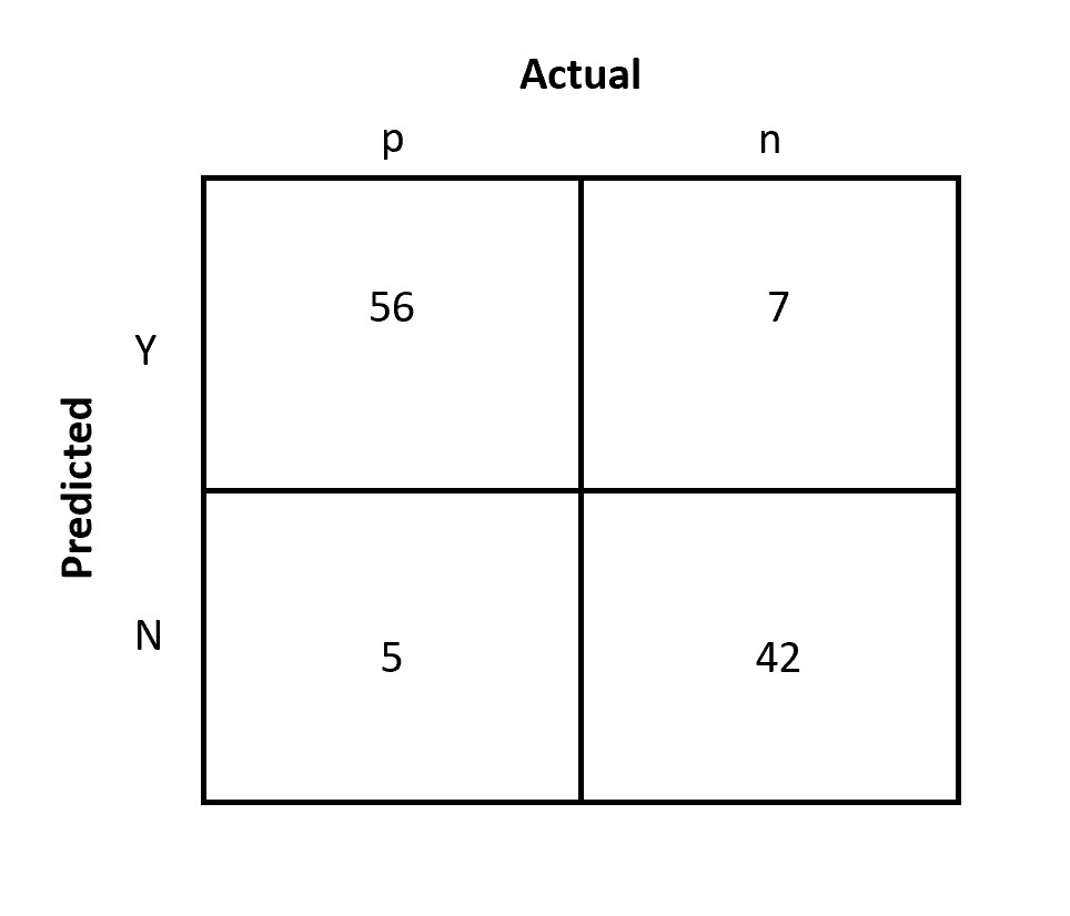
A Data Scientist has trained a Machine Learning model which can tell if they can give a 30% discount on orders to the customer or not. For simplicity, I have split my dataset into training and test dataset. And below is the confusion matrix that I have derived on the test dataset:

Now we know the probability of the outcomes, next we need to know the cost and benefits of each possible outcome. We have estimated the probabilities from the historical data, but it is not easy (or not possible at all) to calculate the cost and benefits from the historical data.

In our example of a food aggregator, the decision to give a discount to the customer depends on the future orders placed by the customers or engagement with the application offerings.

Cost and Benefits

Cost and benefits are the ultimate goals of any business. To proceed further in the expected value calculations, we need to know the expected cost and benefits from the customers. This is a complex calculation to do and needs deep business expertise. For simplicity, let's assume we have driven the results from the historical trends. (Though historical trends are not always the right representation of the future, we will be discussing in detail costs and benefits in future posts).

Similar to the outcome probabilities representation, we have represented the probability of the outcome as a confusion matrix as shown below:

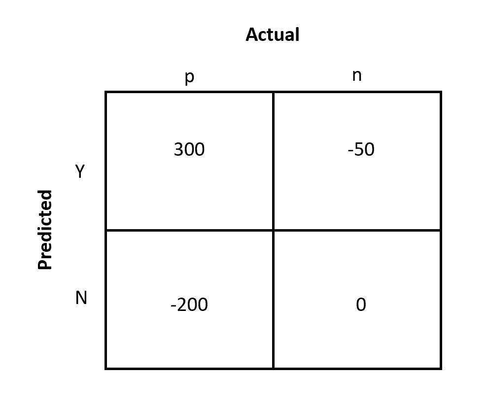
For simplicity, let us assume stakeholders have worked hard and could figure out the marketing expense (INR 50), discounts (30% maximum capped to INR 100), and future benefits from the customers (INR 500). 

The above-shown confusion matrix represents four values as described below:

• False Positive: When we expect customers to be profitable and the customer doesn't respond. In other terms, the cost spent on customers is more than the returns from the customer.
  In this case, the marketing cost is spent on the customer which is INR 50. Since it is money spent therefore represented as b(Y, n) = -50.
   
• False Negative: A potential customer that was not targeted, but would have turned profitable if targeted.
  Since no money is spent and nothing was gained therefore the net impact is 0. But there is an opportunity cost that has to be accounted for. The business has estimated this cost as INR 200. Since the cost is lost therefore the value is represented as b(N, p) = -200.
   
• True Positive: When we expect customers to be profitable and the customer responds.
  The customer was marketed and was given a discount and is expected to turn profitable. So calculations will be, 500 - 50 - 100 = INR 350. Here the net profitability is positive b(Y, p) = 300.
   
• True Negative: A customer that was not targeted, and would have not turned profitable if targeted.
  The customer is not targeted and would have not turned profitable. Therefore net impact is b(N, n) = 0.

Calculating Expected Value

We are all set and have the outcome probabilities and cost and benefits matrix which is needed to calculate the expected value. Let's go further and define the equation of the expected value. This will also solve the puzzle of why cost and benefits are needed to calculate expected value.

The equation of expected value is denoted as

$$EV = p(o_1).v(o_1) + p(o_2).v(o_2) + p(o_3).v(o_3) . . .$$

where \(o_i\) is a possible decision outcome, \(p(o_i)\) is the probability of outcome and \(v(o_i)\) is the value of the outcome. Since we now know both the probability of the outcomes and the profitability in terms of cost and benefits. We can simply plug in the values in the equation to calculate the expected value for this food aggregated business.

Let us rewritten above expected value calculation as per our problem statement needs,

$$EV = p(Y, p).b(Y,p) + p(N,p).b(N,p) + p(N,n).b(N,n) + p(Y,n).b(Y,n)$$

This is one of the straightforward ways to calculate the expected profits. We can directly plugin values and calculate the expected value.

But let us proceed forward and look at the alternative way of calculating the expected value which is often used in practice. We will be rewriting the equation to factor out class priors which help in operating out the influence of class imbalance on the expected value.

A rule of probability states that, 

$$p(x,y) = p(y).p(x/y)$$

Let us update our equation of expected value using this rule,

$$EV = p(Y|p).p(p).b(Y,p) + p(N|p).p(p).b(N,p) + p(N|n).p(n).b(N,n) + p(Y|n).p(n).b(Y,n)$$

After rearranging the above equation,

$$EV = p(p) . [p(Y|p).b(Y,p) + p(N|p).b(N,p)] + p(n). [p(N|n).b(N,n) + p(Y|n).b(Y,n)]$$

Here, we can see that we have two components where first one represents the expected profit from positive scenarios and second one represents the expected profit from negative scenarios. If there is a class imbalance, the contribution of the imbalanced class towards the expected value calculation will be very low.

Further quantities such as \(p(Y|p)\), \(p(Y|n)\), etc. can be calculated directly from the confusion matrix as true positive rate, false-positive rate, etc.

As we can see in the confusion matrix, total observations are 110 out of which 61 (56 + 5) are positive and 49 (7 + 42) are negative. Therefore p(p) = 0.55 and p(n) = 0.45.

Therefore, tp rate p (Y | p) = 56/61 = 0.92; fp rate p (Y | n) = 7/49 = 0.14; fn rate p (N | p) = 5/61 = 0.08; tn rate p (N | n) = 42/49 = 0.86

Substituting the values into the equation,

= 0.55 * (0.92 * 300 + 0.08 *  -200 ) + 0.45 * (0.86 * 0 + 0.14 * -50 )

= INR 138.85

The above-stated expected value means that, if we apply this model to the population data we can expect to see a profit of INR 138.85 per customer.

The expected value is critical as it summarizes the whole complex confusion matrix to a single number but this can be dangerous as well because a lot of conditions can be hidden behind the number. The choice should be yours!!!!