Unlocking the Power of Naive Bayes Algorithm for Text Classification

Naïve Bayes is a popular algorithm that finds use cases in text classification problems. This post will look at example text-related problems and understand how the Naïve Bayes algorithm can help solve problem statements. In general, Naïve Bayes performs well in text classification applications.

This article assumes that you have a basic knowledge of how the Naïve Bayes algorithm work. If you don't know or want to revise the concept, I recommend you go through the Naïve Bayes Algorithm Detailed Explanation article before proceeding further.

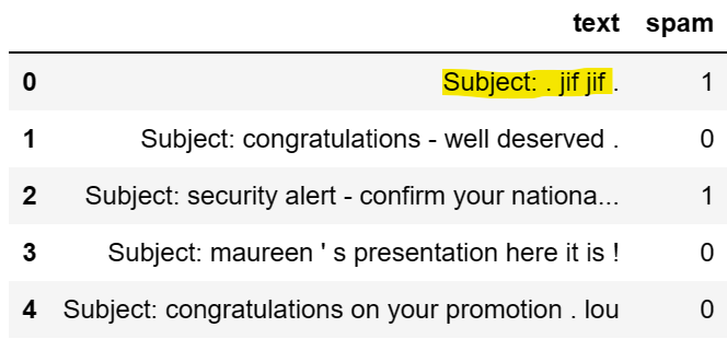
Let us take a problem statement and dataset to proceed forward. The goal here will be to classify text into target variables. For simplicity, we will take 5 random documents from the dataset to understand how the Naïve Bayes algorithm can be used in text classification problems. Below is the dataset that we will be considering in our post.

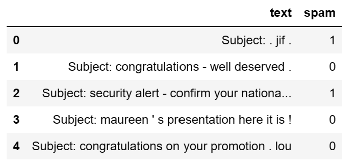
The sample dataset shown above is from the Kaggle Email spam dataset. In this dataset, the text sent over the mail is given along with the label stating either the email is spam (represented as 1) or ham (represented as 0). The task here is to predict if given a new email, classify the email into spam or ham.

The challenge here is that the email column is a collection of words that cannot be directly fed into the Machine Learning algorithm. This is where the Naïve Bayes algorithm comes in handy and helps solve text classification problems.

Preprocessing

Let us start with doing basic preprocessing on the dataset. We have the documents, and we need to convert documents to features on top of which we can train our Naïve Bayes classifier.

Let us start by understanding the vocabulary of the dataset. For the sample dataset containing five emails labeled as spam or ham, there are 28 words, as shown below:

's', '-', 'union', 'national', 'maureen', 'confirm', 'here', '.', 'security', 'alert', 'credit', 'presentation', 'Subject', 'on', '>', 'is', 'lou', 'deserved', '!', ':', 'information', "'", 'your', 'promotion', 'it', 'well', 'congratulations', 'jif'

Out of the words, let us first remove the stop words from the list. After removing stop words, we are left with 15 words, as stated below:

'alert', 'confirm', 'congratulations', 'credit', 'deserved', 'information', 'jif', 'lou', 'maureen', 'national', 'presentation', 'promotion', 'security', 'subject', 'union'

The following stop words are removed from the vocabulary of the words we were having earlier:

's', '-', 'here', '.', "'", 'your', 'it', 'well', 'subject', 'Subject', 'on', '>', 'is', '!', ':'

Once we have stop words removed, let's create a bag of words. It is the simplest technique available to convert documents to features that can be used to train a machine-learning algorithm. Simply stated, In the bag of words technique, we use the vocabulary/dictionary to represent the given test documents by counting the occurrences of various words.

Let us represent the words we obtained after removing the stop words in the bag of words representation.

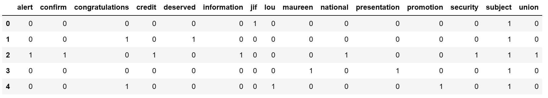
In the diagram above, we can observe five rows representing the document from our sample dataset. The column value represents the occurrence of the words in the document.

E.g., If we consider our first document, "Subject: . jif .", after removing the stop words, we are left with "Subject jif" and the first row of the bag of words representation has a value of 1 for columns "Subject" and "jif".

Let us represent the bag of words in array format and differentiate them based on the class spam or ham.

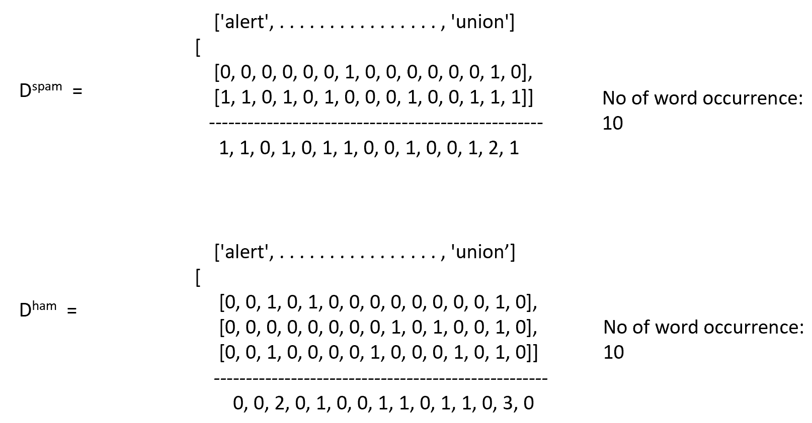
In addition to dividing documents into spam or ham, we have also calculated the total occurrence of each word for the document's different classes (spam and ham). The order of the words represented in the array above is as follows:

'alert', 'confirm', 'congratulations', 'credit', 'deserved', 'information', 'jif', 'lou', 'maureen', 'national', 'presentation','promotion', 'security', 'subject', 'union'

We performed our pre-processing steps and represented the data in a format that can be easily used for a Naïve Bayes algorithm. This post will primarily focus on Multinomial Naïve Bayes Classifier and Bernoulli Naïve Bayes Classifier.

Let's start with the Multinomial Naïve Bayes Classifier and learn how the algorithm's training takes place.

Multinomial Naïve Bayes Classifier

Now we have converted documents into features, let's understand how we can use a Naïve Bayes classifier to classify the documents into target classes.

The very first step is to calculate the prior and likelihood probabilities. The reason behind such a calculation is that we can classify any new document into the target class using prior and posterior probabilities.

Let us start by calculating the prior probabilities. Let us consider our sample dataset where we have 5 documents, of which 2 are spam and 3 are ham. Therefore our prior probabilities will be \(p(spam) = 2/5\) and \(p(ham) = 3/5\).

Our goal is to classify the new document into spam or ham class. We can apply Bayes Theorem for such a calculation as following:

$$P(spam | w_1, w_2, ........ w_n) = {P(w_1, w_2, ........ w_n | spam) * p(spam) \over P(w_1, w_2, ........ w_n)}$$

where \(P(spam)\)  represents the prior probabilities, \(P(w_1, w_2, ........ w_n | spam)\) represents likelihood probabilities and \(P(spam | w_1, w_2, ........ w_n) \) represents the posterior probabilities.

Here we are calculating the probability of the document being spam, given the words in the new document. Similarly, we can calculate the probability of a document being ham given the word as follows:

$$P(ham | w_1, w_2, ........ w_n) = {P(w_1, w_2, ........ w_n | ham) * p(ham) \over P(w_1, w_2, ........ w_n)}$$

Now comparing the two probabilities, we can classify the new document into spam or ham.

We have already calculated the probability of  p(spam) and p(ham), therefore only the calculation of likelihood probabilities

$$P(w_1, w_2, ........ w_n | class)$$

is pending where class represents spam or ham. Let us consider spam class and further simplify the representation of the likelihood probabilities as

$$P(w_1|spam) * P(w_2|spam) *  . . . . . . . . . . . * P(w_n|spam)$$

The probability of the word in a document labeled as spam is easy to calculate using the bag of words representation we have done earlier. But to make understanding much simpler, let us represent the bag of words as a table that can give us direct values for the probability calculation as represented below:

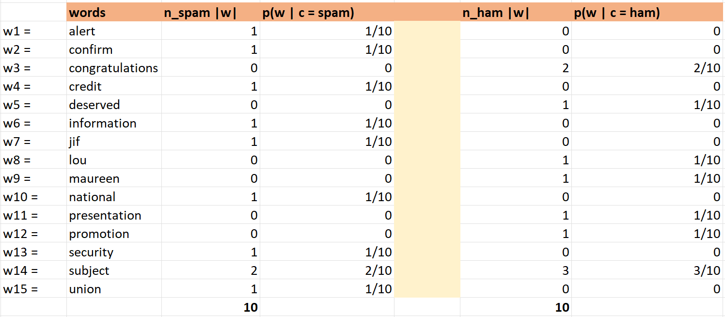
Here in the table shown above, we have represented words and the occurrence of the words in each class (spam and ham), and thereafter we have calculated the probabilities of words given a class.

Now using this, we can classify the new document into a class. And this is the actual classification process used by the Multinomial Naïve Bayes Classifier.

Let's say there is a document "national information", and we want to classify it into spam and ham. We will calculate this as (ignoring the denominator as it will be the same for both class spam and ham):

$$P(spam | national, information) ≈ P(national, information | spam) * p(spam)$$

which can be further simplified as,

$$P(spam | national, information) ≈ P(national | spam) * P(information | spam) * p(spam)$$

Now, this can be calculated easily from the table above,

$$P(spam | national, information) ≈ 1/10 * 1/10 * 2/5 = 0.004$$

Similarly, we can calculate the probability that a document is a ham.

$$P(ham | national, information) ≈ P(national | ham) * P(information | ham) * p(ham) = 0 * 0 * 3/5 = 0$$

Now comparing the probabilities, we can classify the document. But here, we have observed that the probability of the document being a ham is calculated as 0.

This happens because words in the document have 0 probability for a given class, i.e., ham in our example. In such a case, since we are multiplying the probabilities, the whole expression turns to 0.

How do you deal with such a problem? To solve a problem, we use the concept of Laplace smoothing. Let us understand further to understand.

Laplace Smoothing

Using this technique, we increment the occurrence of words by 1 or alpha. Let us recalculate the table that can give us direct values for the probability calculation again, as represented below:

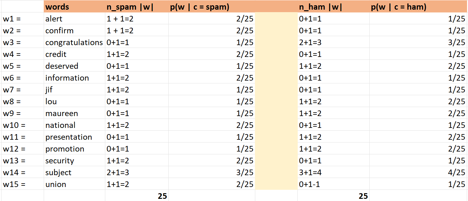
Here we added 1 to the occurrence of every word so that our probabilities never return to 0. After adding Laplace smoothing, we recalculated the probabilities again.

Let us classify the document "national information" again that we have seen earlier, where the probability term was zero.

$$P(spam | national, information) ≈ P(national | spam) * P(information | spam) * p(spam) = 2/25 * 2/25 * 2/5 = 0.003$$

And,

$$P(ham | national, information) ≈ P(national | ham) * P(information | ham) * p(ham) = 1/25 * 1/25 * 3/5 = 0.001$$

Therefore we classify the document as spam.

Suppose we have a new document, "super national information" with the word "super" that doesn't exist in our vocabulary. How do we calculate the likelihood probabilities in this case?

We ignore such words that are not present in the vocabulary and proceed in the same manner as shown above.

The whole of the above calculation can be easily performed using Python packages. Let us see a pseudo python code to classify the document using Multinomial Naïve Bayes Classifier.

from sklearn.model_selection  import train_test_split
from sklearn.naive_bayes import MultinomialNB
from sklearn import metrics

X_train, X_test, y_train, y_test = train_test_split(df['text'], df['class'], random_state=1)

coun_vect = CountVectorizer(stop_words='english')
vect = coun_vect.fit(X_train)

# transforming the train and test datasets
X_train_transformed = vect.transform(X_train)
X_test_transformed = vect.transform(X_test)

# Observe Bag of words representation
count_array = X_train_transformed.toarray()
features = coun_vect.get_feature_names()

# create DataFrame as a bag of words
df_bow = pd.DataFrame(data=count_array, columns=features)


mnb = MultinomialNB()
mnb.fit(X_train_transformed,y_train)

# predict class
y_pred_class = mnb.predict(X_test_transformed)
y_pred_proba = mnb.predict_proba(X_test_transformed)

# Evaluation
metrics.accuracy_score(y_test, y_pred_class)

Bernoulli Naïve Bayes Classifier

Till now, we have been exploring the multinomial way of classifying documents. The most fundamental difference in Bernoulli Naïve Bayes Classifier is how we build the bag of word representation, which is just 0 or 1. Bernoulli's Naïve Bayes is concerned only with whether the word is present or not in a document. In contrast, Multinomial Naïve Bayes counts the no. of occurrences of the words.

Let us consider the first row of the sample dataset that we considered earlier, having the text "Subject: . jif .". Let's update this text to "Subject: . jif jif ." and see how the bag of word representation changes.

Now, let us represent a bag of word representation for the above-updated dataset where a word appears twice in the document for solving classification problems using Multinomial Naïve Bayes and Bernoulli Naïve Bayes.

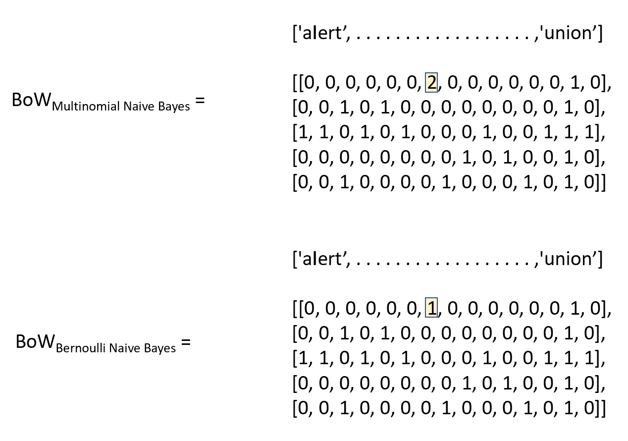
The order of the words represented in the array above is still the same as represented earlier:

'alert', 'confirm', 'congratulations', 'credit', 'deserved', 'information', 'jif', 'lou', 'maureen', 'national', 'presentation','promotion', 'security', 'subject', 'union'

The only difference is for the word "jif" in the first document, as it has appeared twice in the document.

Pseudo python code to classify the document using Bernoulli Naïve Bayes Classifier.

from sklearn.model_selection  import train_test_split
from sklearn.naive_bayes import MultinomialNB
from sklearn import metrics

X_train, X_test, y_train, y_test = train_test_split(df['text'], df['class'], random_state=1)

coun_vect = CountVectorizer(stop_words='english')
vect = coun_vect.fit(X_train)

# transforming the train and test datasets
X_train_transformed = vect.transform(X_train)
X_test_transformed = vect.transform(X_test)

bnb = BernoulliNB()
bnb.fit(X_train_transformed,y_train)

# predict class
y_pred_class = bnb.predict(X_test_transformed)
y_pred_proba =bnb.predict_proba(X_test_transformed)

# accuracy
metrics.accuracy_score(y_test, y_pred_class)

The above code is an example of using the Bernoulli Naïve Bayes algorithm for text classification using the scikit-learn library in Python. The dataset is preprocessed using the CountVectorizer and then trained using the BernoulliNB classifier. The model is then tested on test data, and the predictions are made.

Conclusion

In conclusion, the Naïve Bayes algorithm is a powerful tool for text classification that utilizes the Bayes theorem to make predictions based on prior knowledge and evidence. Its simplicity and effectiveness have been widely used in various applications such as spam detection, sentiment analysis, and language modeling.

By understanding the key concepts and implementation of the algorithm in Python using Multinomial and Bernoulli Naïve Bayes, we can easily apply it to our projects and improve the accuracy of our predictions. Overall, the Naïve Bayes algorithm is a valuable addition to any data scientist or machine learning enthusiast's toolkit.