Support Vector Machines Detailed Explanation

There are a lot of algorithms like logistic regression, Naive Bayes, etc that are used to solve classification problems. Though these algorithms are popular and used across the industry, they fail to classify complex classification tasks like image classification, voice detection, etc.

Support Vector Machines are also known as SVM which are capable of dealing with quite complex problems, where models like logistic regression mostly fail. A few of the properties and use cases of the SVM algorithm are:

1. SVMs are mostly used for classification tasks, but they can also be used for regression. 
2. It has the ability to deal with computationally heavy data sets, classify non-linearly separable data, etc.
3. SVMs are also linear models as they belong to the class of linear machine learning models (logistic regression is also a linear model).
4. SVMs need attributes in the numeric form. If our features are non-numeric in the dataset, we need to convert them to numeric first.

Here in this post, we will be learning the SVM algorithm as the classification algorithm. Before we move to understand support vector machines, let's spend some time understanding the concept of hyperplanes.

Hyperplanes

In the context of data, a hyperplane is a boundary that divides data into two different parts. We can have a hyperplane in 2 dimensions, 3 dimensions, or let's say n dimension plane as well, which is beyond our imagination.

In 2 dimension the hyperplane or line will be represented by:

ax +  by + c = 0

In 3 dimension the hyperplane will be represented by:

ax +  by + cz + d = 0

Or, In general in n-dimensional, the hyperplane will be represented as:

$$\sum_{i = 1}^d(W_i . X_i) + W_0 = 0$$

The model denoted by the expression given above is called a linear discriminator.

Linear Discriminator states that we need to find the coefficients \(w_1\) to \(w_d\) including \(w_o\) in such a way that below condition holds true for every data point:

if \(l_i = 1\) then: $$\sum_{i = 1}^d(W_i . X_i + W_0) > 0$$

if \(l_i = -1\) then: $$\sum_{i = 1}^d(W_i . X_i + W_0) < 0$$

The above condition states that we need to find coefficients of a hyperplane in such a way that all data points of one class remain on one side and all other data points of another class remain on another side of the hyperplane.

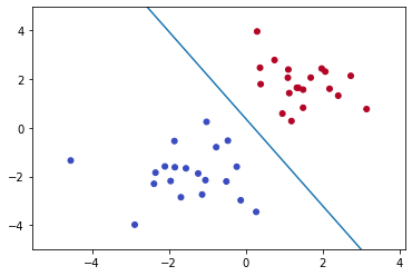
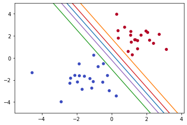
Great till now. But there is an issue: There could be multiple possible planes that could satisfy Linear Discriminator. So how to find out the best hyperplane?

Maximal Margin Classifier

The Maximal Margin Classifier ensures the margin of safety. It divides the data set in such a way that it is equidistant from both classes. Thus, it maintains an equal distance from both classes, making the model less biased toward the training data. Also, training errors are reduced.

The best line is the one that maintains the largest possible equal distance from the nearest points of both classes. The points that lie close to the plane are called Support vectors. These are the only points that are used in constructing the hyperplane.

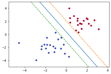
Goal: We are trying to find the weights of the model such that the margin to the points nearest to the hyperplane is maximum.

Prerequisites:

Here, I am assuming that you are well known of the mentioned concepts:

1. Dot Product of two vectors
2. Distance Formula for a Hyperplane

To find the maximum margin the points to consider are support vectors. Our task is to find a plane that is at the maximal distance from the support vectors. So our problem gets reduced to where we need to find the weights corresponding to the hyperplane having the maximum possible margin.

Mathematical to find the maximum margins from the hyperplane we will be calculating the distance of the point to the hyperplane. The mathematical formulation requires two major constraints that need to be taken into account while maximizing the margin:

1. The standardization of coefficients such that the summation of the square of the coefficients of all the attributes is equal to 1. i.e: \(\sum_{i = 1}^d(W_i^2)  = 1\)
2. The maximal margin hyperplane should also follow the constraint:  \( (l_i * (W_i.Y_i)) \geq M\) 

Maximal Margin Classifier address the limitation of the hyperplane by adding margins. But in real-world data is not symmetric and there will be few points that will be lying on the wrong side of the plane.

In such scenarios, Maximal Margin Classifier will not work and we need to think of an alternative which is the Soft Margin Classifier or Support Vector Classifier.

Soft Margin Classifier or Support Vector Classifier

In the real world datasets most of the time it is not possible to draw a hyperplane that splits two classes. In such cases, we use Soft Margin Classifier.

The hyperplane that allows certain points to be deliberately misclassified is also called the Support Vector Classifier. 

The support vector classifier works well when the data is partially intermingled (i.e. most of the data can be classified correctly with some misclassifications).

Similar to the Maximal Margin Classifier, the Support Vector Classifier also maximizes the margin; but it will also allow some points to be misclassified.

Slack Variables help to control the misclassification in the Support Vector Classifier. Let's understand the slack variable in detail.

Slack Variable

Slack is the tolerance that we allow for every data point. It tells us where an observation is located relative to the margin and hyperplane. As we have seen in Maximal Margin Classifier to maximize the margin constraint is given by:

$$l_i * (W_i.Y_i) \geq M$$

In the case of the Support Vector Classifier, the constraint remains almost the same. The only difference is slack variable is added.

$$l_i * (W_i.Y_i) \geq M(1-\epsilon_i)$$

where \( \epsilon_i\) represent's the slack variable.

Below are the properties of the slack variable:

• For points that are at a distance of more than M, i.e. at a safe distance from the hyperplane, the value of the slack variable is 0. 
• If a data point is correctly classified but falls inside the margin (or violates the margin), then the value of its slack ϵ is between 0 and 1.
• If a data point is incorrectly classified (i.e. it violates the hyperplane), the value of epsilon (ϵ) > 1.

So, every data point will be having a slack variable associated with it. And the summation of the slack variable is represented as the cost of the model (C).

$$\sum\epsilon_i \leq C$$

The higher the cost of the model states that there are many points misclassified. And the model is generalized and less likely to overfit. In other words, the model has a high bias.

And lower the cost of the model states that there is less number of points misclassified. And the model is less generalized and more likely to overfit. In other words, the model has a high variance.

So by now, you might have guessed C is the hyperparameter of the SVM model and needs to be tuned to control the misclassification of the model.

So far we have understood the concepts of the Maximal Margin Classifier and the Support Vector Classifier. Both of them tend to fit the hyperplane to separate the classes.

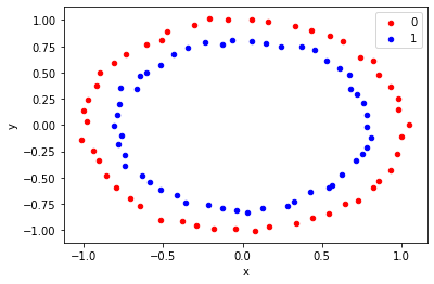
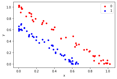
But most of the real-world datasets are nonseparable with the help of Linear boundary. So how should we classify nonlinear datasets? Consider an example showing a nonlinear dataset:

from sklearn.datasets import make_circles
import matplotlib.pyplot as plt
from pandas import DataFrame

# generate 2d classification dataset
X, y = make_circles(n_samples=100, noise=0.02)

# scatter plot, dots colored by class value
df = DataFrame(dict(x=X[:,0], y=X[:,1], label=y))
colors = {0:'red', 1:'blue'}
fig, ax = pyplot.subplots()
grouped = df.groupby('label')

for key, group in grouped:
    group.plot(ax=ax, kind='scatter', x='x', y='y', label=key, color=colors[key])
pyplot.show()

OUTPUT:

Kernels

Kernels enable SVM models to serve the purpose of classifying nonlinear datasets. Kernel works on an algorithm for mapping nonlinear data to linear data. Wondering how? Let's look at it next.

Converting nonlinear data to linear

Let's go back to the basics. We know each and every point in 2D is plotted in the X and Y plane/space.

Now consider a dataset that is nonlinear in X and Y space. Now, what if we find a function and apply it to the dataset in X and Y space to make it linear in the new space X' and Y'.

Amazing trick! What do you guys think?

NOTE: The original space (X, Y) is called the original attribute space, and the transformed space (X’, Y’) is called the feature space. And the process of transforming the original attributes into a new feature space is called feature transformation.

Let's consider an example of concentric circles that we have seen earlier. And transform nonlinear function to linear function in feature space.

from sklearn.datasets import make_circles
import matplotlib.pyplot as plt
from pandas import DataFrame

# generate 2d classification dataset
X, y = make_circles(n_samples=100, noise=0.02)

X[:,0] = pow((X[:,0] - 0.01), 2)
X[:,1] = pow((X[:,1] - 0.01), 2)

# scatter plot, dots colored by class value
df = DataFrame(dict(x=X[:,0], y=X[:,1], label=y))
colors = {0:'red', 1:'blue'}
fig, ax = pyplot.subplots()
grouped = df.groupby('label')
for key, group in grouped:
    group.plot(ax=ax, kind='scatter', x='x', y='y', label=key, color=colors[key])
pyplot.show()

OUTPUT:

As we have seen above we can visualize the transformation happening.  But in real-world datasets, we have a lot of features, and almost impossible to transform data.

Consider a scenario where I have a dataset close to a circle in two-dimension space. So I know I want to transform to degree 2. Therefore my feature set would be:

$$ax^2 + by^2 + cxy + dx + ey + fc = 0$$

My feature space grows to 6 dimensions from 2 dimensions. What if I have 100+ features and I need to transform them to 2 degrees or higher? Computationally it's an expensive operation to perform.

Let's see how kernel addresses these problems:

1. Transforming non-linear data to linear data.
2. Computational power needs for the non-linear transformation.

The kernel is a black box where the input is the original attributes and output is the transformed attributes in higher dimension space. 

We can think of a kernel as a function that helps us to transform nonlinear data implicitly. Then the SVM algorithm uses a transformed attribute generated from the kernel to generate a classifier as usual.

NOTE: Here the kernel is also responsible for mapping transformed feature space to the actual feature space as well.

Kernel Trick Revealed

The kernel doesn't perform transformation explicitly but uses a mathematical hack to perform the transformation.

Suppose there is function ϕ which transforms high dimension non-linear data to the linear space. We calculate the pairwise inner products of the feature vectors \(\phi (X_i^T).\phi (X_j)\), using which the learning algorithm can build a model in the linear feature space.

The next huddle is where we need to find out ϕ which can help us to do the transformation. This is where kernel tricks come in. 

Where instead of finding a dot product of feature vectors \(\phi (X_i^T).\phi (X_j)\), we define a function K whose value is equal to the dot product of feature vectors.

$$K(\vec x_i, \vec x_j)  \equiv \phi (X_i^T).\phi (X_j)$$

where k is popularly known as kernel functions. There are various types of kernel functions. Let's understand them next.

Types of Kernel

Now that we have a detailed understanding of the kernel and why we need it, let's dig further and explore the different types of kernel functions available:

1. The linear kernel
2. The polynomial kernel
3. The radial basis function (RBF) kernel

Let's understand them in detail.

The linear kernel

This is the same as the support vector classifier, or the hyperplane, without any transformation at all. It is used when we can draw a linear plane to separate two classes without performing any transformation. 

$$(\vec x_i^T. \vec x_j)$$

The sklearn package has one tunning parameter in the case of linear kernel i.e. Cost (C).

The polynomial kernel

It is capable of creating nonlinear, polynomial decision boundaries. The kernel function is represented as

$$(\vec x_i^T. \vec x_j + \theta)^d$$

where d represents the degree of the polynomial. Also, theta and d are the hyperparameters.

The radial basis function (RBF) kernel

This is the most complex one, which is capable of transforming highly nonlinear feature spaces into linear ones. It is even capable of creating enclosed decision boundaries. The kernel function is represented as

$$e^{- \alpha || \vec x_i. -\vec x_j||^2}$$

The sklearn package has two tunning parameters in the case of RBF kernel:

• Cost: The cost of the model
• gamma: It controls the amount of non-linearity in the model - as gamma increases, the model becomes more non-linear, and thus model complexity increases.

RBF is one of the popularly used kernel functions.

NOTE: 

• Please note that choosing the right kernel and tunning hyperparameter correctly is very important. Failing to do will result in either the overfitting or naive model.
• We generally use cross-validation to tune hyperparameters (Cost and Gamma) and hit and trial to choose between polynomial and RBF kernel.

Apart from the mentioned kernel functions, there are other types as well like Gaussian Kernel, Sigmoid Kernel, Spectrum Kernel for string, etc.

Loss Function

Support vector machines use hinge loss function. It is a function that incurs no penalty for the data points that are on not on the wrong side of the margin. The loss function only becomes positive (or incurs a penalty) when the data points are on the wrong side of the boundary and beyond the margin.

The hinge loss function also increases linearly as the data points are farther away on the wrong side of the boundary. In other terms, data points are penalized if they appear on the wrong side, and additionally the penalty increases if they are further away from the boundary.

Another not soo popular loss function that can be used is zero-one loss. As the name suggests, it assigns zero for correct decisions and one for incorrect decisions.

Summary

Here we discussed why we need the SVM algorithm. We also discussed Hyperplanes, Maximal Margin Classifiers, and Soft Margin Classifiers. We introduced the slack variable and discussed how it can help to classify real-world data.

We understand how the kernel trick works, where we concluded that the key fact that makes the kernel trick possible is that to find the best fit model, the learning algorithm only needs the inner products of the observations \(X_i^T.X_j\).