Principal Component Analysis Detailed Explanation

Principal Component Analysis (PCA) is a powerful statistical technique for dimensionality reduction and data visualization. PCA allows us to transform high-dimensional data into a lower-dimensional space while retaining most of the original variance in the data. This makes it easier to visualize, analyze and model complex datasets.

However, understanding the mathematical concepts and intuition behind PCA can be challenging for beginners. This post will explain Principal Component Analysis, including the underlying mathematics and practical implementation. By the end of this post, readers will have a comprehensive understanding of Principal Component Analysis.

Prerequisites

Before learning Principal Component Analysis (PCA), it is recommended to have a solid understanding of the following prerequisite concepts:

• Matrix: Before understanding PCA, it's essential to understand the fundamental matrix as PCA starts with a matrix of data, typically represented as n rows (observations) and p columns (variables).

• Linear algebra: PCA involves matrix operations such as eigendecomposition, singular value decomposition (SVD), and matrix multiplication. Knowledge of linear algebra concepts such as matrix operations, linear combinations, linear transformation, eigenvectors, and eigenvalues will help understand PCA.

• Multivariate statistics: PCA is a multivariate statistical technique used to reduce the dimensionality of data. A basic understanding of statistical concepts such as covariance, correlation, and variance will help understand the intuition behind PCA.

• Data preprocessing: PCA assumes that the data is normalized and standardized, so it is crucial to have a good understanding of data preprocessing techniques such as scaling, centering, and normalization.

A good grasp of these concepts will provide a strong foundation for learning and understanding Principal Component Analysis. In this post, I will start by summarizing a few of the prerequisites needed to understand the depth of the post. Let's get started.

Matrix

A matrix is a rectangular array of numbers, symbols, or expressions arranged in rows and columns. In linear algebra, matrices represent linear transformations between vector spaces.

Below is the summary of the different types of matrices available, as this post assumes that the reader has prior knowledge about the matrix.

• Null Matrix: A matrix that has all elements 0 is called a null matrix
• Row Matrix: A row matrix is a matrix with only one row
• Column Matrix: A column matrix is a matrix with only one column
• Square Matrix: A matrix is considered square if it has the same number of rows as columns.
• Diagonal Matrix: A diagonal matrix is a square matrix where all the elements are 0 except those in the diagonal from the top left to the bottom right corner. 
• Identity Matrix: The identity matrix is a square matrix with 1's along the main diagonal and 0's for all other entries.
• Symmetric Matrix: A matrix whose transpose is the same as the original matrix is called a symmetric matrix.
• Orthogonal Matrix: A matrix A is orthogonal if \(𝐴𝐴^𝑇 = 𝐴^𝑇𝐴 = I\).
• The determinant of a Matrix: It can be viewed as a function whose input is a square matrix and whose output is a number.
• Transpose of a Matrix: The transpose of a matrix is created by converting its rows into columns; that is, row 1 becomes column 1, row 2 becomes column 2, etc.
• The inverse of a Matrix: For a square matrix A, the inverse matrix \(𝐴^{−1}\) is a matrix that, when multiplied by A, yields the identity matrix of the vector space. i.e., \(𝐴𝐴^{−1} = I\).

Linear Combination

A linear combination of a set of vectors is an expression obtained by multiplying those sets of vectors with a scalar/actual number and then adding them up. For example:

v1 = np.array([2,3])
v2 = np.array([3,4])
m = 1
n = 2

lincom = m*v1 +  n*v2
print(lincom)

# The linear combination vector would, therefore, be shown as (2m + 3n, 3m+ 4n)

We can do the reverse part as well. That is, finding the values of m, n for which the given vector is a linear combination of the previous two vectors.

lincom2  = ([8,11])
setvec = np.array([[2,3],[3,4]])
m,n = np.linalg.solve(setvec, lincom2)
m,n

We can try this and represent any vector in 2 Dimension space as the linear combination of the vector (2,3) and (3,4). But this will not hold for any combination of the vector. Consider an example:

We cannot represent any vector as a linear combination of vectors (2,0) and (3,0). This is because (2,0) and (3,0) are collinear vectors. i.e., one of the vectors can be represented as a scalar multiple of the other vector (3,0) = 1.5(2,0).

Collinear vectors always have the same direction and can always be represented as scalar multiples of one another.

Basis Vector

Given a set of vectors where no matter what other vector we pick, it can always be represented as a linear combination of the given set, then given vectors are known as the basis vectors for that data space or dimension.

# Verifying (2,3) and (3,4) are basis vector
lincom2  = ([6,3])
setvec = np.array([[2,3],[3,4]])
m,n = np.linalg.solve(setvec, lincom2)
round(m),round(n)

There are a few properties of the standard basis vector ( i(1,0) and j(0,1) ). These are:

1. It is orthogonal, i.e., the vectors (1,0) and (0,1) are perpendicular.

   ## Dot products of perpendicular vectors are always zero
   setvec = np.array([[1,0],[0,1]])
   np.dot(setvec[0],setvec[1])

2. It is normalized, i.e., the magnitude of each vector is 1. i.e., \(\sqrt{(1^2 + 0^2)}\) = 1​

   ##This would mean that each of them would be of unit magnitude
   np.linalg.norm(setvec[0])
   np.linalg.norm(setvec[1])

Linear Transformation

A linear transformation is a matrix transformation on a vector where the vector's geometric properties change due to elongation, rotation, shifting of axes, or some other form of distortion.

If L is a matrix that denotes the transformation and v is the vector on which the transformation is happening, then the resultant vector is given by Lv. There is a different types of transformations that can be performed, as discussed below.

Elongation

Let's see how multiplying a vector/matrix with another vector elongates it. Let's consider a linear transformation where the original basis vectors i(1,0) and j(0,1) move to the points i'(2,0) and j'(0,1).

# Dataframe matrix
a = [[1,2],[-2,3],[-2,1],[3,7],[4,5],[6,4]]
b = ['X','Y']
c = pd.DataFrame(a,columns = b)

# Linear transformation matrix
L = np.array([[2,0],[0,1]])

# Let's apply the transformation now to every vector in the data frame
# We are taking transpose so that transformation happens on each vector
d  = L @ (c.values).T
print(d.T)

# Output
array([[ 2,  2],
       [-4,  3],
       [-4,  1],
       [ 6,  7],
       [ 8,  5],
       [12,  4]], dtype=int64)

The reason for taking (c.values).T over here is because over original vectors represented in the Data Frame format are in row format. But for transformation to work, we need the vectors and columns.

In the example shown above, we have performed elongation on the DataFrame, where we have extended 'X' values by 2 an' 'Y' values by 1 by performing the dot product of the transformation matrix to the original matrix.

Shifting of axis

Let's say we have an example where we want to shift a vector (1,1) from the origin from the original coordinate system (0, 0) to the new origin (2,2). The below python code demonstrates the implementation.

import numpy as np

# Define a vector in the original coordinate system
v = np.array([1, 1])

# Define the new origin
origin = np.array([2, 2])

# Shift the origin of the vector
v_shifted = v - origin

# Print the results
print("Original vector:", v)
print("Shifted vector:", v_shifted)

This example defines a vector v in the original coordinate system and a new origin. We then shift the origin of the vector by subtracting the origin from v, storing the result in v_shifted. The output of the program shows the original and shifted vectors.

Further types of linear transformations can be applied to a vector: Basis Transformation and Space Transformation.

Basis Transformation

A basis transformation involves changing the basis vectors of a vector space while keeping the vectors in the space fixed. This means that every vector in the space can be represented as a linear combination of the new basis vectors. This linear combination's coefficients may differ from those in the old basis. Let's say from the original basis vectors i(1,0) and j(0,1), and we want to shift it to the new orthonormal basis vector i'(0.8,0.6) and j'(-0.6,0.8). 

L = np.array([[0.8,-0.6],[0.6,0.8]])

# Finding the inverse to transform the basis vector
Ld = np.linalg.inv(L)


a = [[1,2],[-2,3],[-2,1],[3,7],[4,5],[6,4]]
b = ['X','Y']
# Data points representation in old basis
c = pd.DataFrame(a,columns = b)

# Transform the vector to the new basis
d  = Ld @ (c.values).T
# Or, np.dot(Ld, (c.values).T)

print("Old basis matrix:", c)
print("New basis matrix:", d.T)

One common question is, why have we taken the inverse of the transformation matrix?

In the python code shown above, we perform transformation 'L' and want to calculate the new matrix d, such that \(L.d = c\). In other words, after applying the transformation to the new matrix, we want to calculate a matrix that equals the original matrix.

To find the matrix d from equation \(L.d = c\), let us multiply \(L^{-1}\) on both side,

$$L^{-1}L.d = L^{-1}c$$

From the inverse of the matrix property, we know that \(L^{-1}L = I\) and any matrix multiply by identify matrix returns the original matrix. Therefore, we can calculate matrix 'd' as,

$$d = L^{-1}c$$

which is the same calculation performed above.

Space Transformation

On the other hand, in space transformation, the origin and the data points change their locations. They remain fixed in the space. However, the representation of the point on the new vector space changes.

import numpy as np

# Define a linear transformation matrix
A = np.array([[1, 2], [3, 4]])

# Define a vector in the original space
v = np.array([1, 1])

# Apply the transformation to the vector
v_transformed = np.dot(A, v)

# Print the results
print("Original vector:", v)
print("Transformed vector:", v_transformed)

This example defines a linear transformation matrix A and a vector v in the original space. We apply the transformation to v using matrix multiplication, storing the result in v_transformed. The output of the program shows the original and transformed vectors.

NOTE: The elongation that we have discussed above is the type of space transformation. The two concepts are not interchangeable and refer to different aspects of geometric transformations.

While these concepts of axis shifting, basis transformation, and space transformation are related and may be used together in certain situations, they have distinct meanings and should not be confused.

Eigendecomposition, Eigenvectors and Eigenvalues

Eigendecomposition is a part of linear algebra that we use for factoring a matrix into its canonical form. After factorization using the eigendecomposition, we represent the matrix in terms of its eigenvectors and eigenvalues.

A special kind of linear transformation that can happen to a vector is that when a matrix is multiplied by it, it only manages to stretch the vector by a certain scalar magnitude. These vectors are known as eigenvectors for that particular matrix, and that scalar magnitude is known as the corresponding eigenvalue. Formally, they can be written as follows,

Av = λv, where A is the original matrix, v is the eigenvector, and λ is the corresponding eigenvalue.

Consider an example shown below calculating eigenvalues and eigenvectors:

A = np.array([[2,1],[1,2]])

K = np.linalg.eig(A)

#Eigenvalues
print(K[0])

#Eigenvectors
print(K[1])

# Verify the results
# Let's verify them once again. First, let's calculate Av
print(A @ (K[1].T)[0])

#Now let's calculate λv.
3*(K[1].T)[0]

# Output:
# As we can see Av = λv has been verified.

Geometrically, we can say that an eigenvector corresponding to an eigenvalue of any matrix is the vector that the matrix shrinks, and the eigenvalue corresponding to that eigenvector defines the amount of shrink. Let's say that N is a square matrix, then we can factorize N as follows:

$$N = QQ^{-1}$$

Where Q is a square matrix with the dimensions of A X A and its column is an eigenvector of N.  is a diagonal matrix.

The parent matrix can be obtained from the eigenvectors and eigenvalues.

$$A = Q . diag(V) . Q^{-1}$$

where Q is a matrix comprised of the eigenvectors, diag(V) is a diagonal matrix comprised of the eigenvalues along the diagonal (sometimes represented with a capital lambda), and \(Q^{-1}\) is the inverse of the matrix comprised of the eigenvectors.

# Arrange the eigenvalues along the diagonal of a square matrix.
# diag(V)
S = np.array([[3,0], [0,1]])

# Take eigenvector
Q=K[1]

# take the inverse of eigenvector
# Q^-1
P = np.linalg.inv(Q)

# The product of the three matrices obtained in the following order returns the original matrix
Q @ S @ P

Introduction to PCA

After getting the basic knowledge required to understand PCA, let us dig deeper and understand how PCA works.

The motivation behind Principal Component Analysis (PCA) is to reduce the dimensionality of a dataset while retaining as much of the variability in the data as possible. This is important because high-dimensional datasets can be challenging to work with, both computationally and conceptually, leading to overfitting and poor model performance.

PCA achieves this by finding the principal components of the data, which are the linear combinations of the original variables that capture the most variation in the data. By projecting the data onto a lower-dimensional space defined by these principal components, PCA allows for easier data visualization, analysis, and modeling.

Properties of PCA

PCA identifies the principal components of the data, which are the linear combinations of the original variables that capture the most variation in the data. These components are computed such that the first principal component captures as much of the variability in the data as possible, the second principal component captures as much of the remaining variability as possible, and so on.

Each principal component is orthogonal (i.e., uncorrelated) to all of the other principal components, and they are ordered by the amount of variability they capture. They are the linear combination of the original features.

$$Z_1 = \phi_{11} X_1 + \phi_{21} X_2 + . . . . . + \phi_{1n} X_n$$

How PCA works?

Initially, PCA used the eigendecomposition route in finding the principal components. However, much faster algorithms like SVD (we will be discussing SVD later in the post) have emerged, predominantly used nowadays. However, one thing to note here is that SVD is a generalized procedure of eigendecomposition.

I will be putting the learnings together from the eigendecomposition and PCA section and summarize the steps involved in finding the principal components using the eigendecomposition route:

1. From the original matrix that we have, we compute its covariance matrix C
2. After computing the covariance matrix, we perform the eigendecomposition and find its eigenvalues and eigenvectors
3. Sort the eigenvectors based on the eigenvalues
4. These eigenvectors are the principal components of the original matrix and denote the amount of variance explained by the eigenvectors. The higher the eigenvalues, the higher the variance the corresponding eigenvector explains
5. These eigenvectors are orthonormal,i.e., unit vectors perpendicular to each other

We should ponder, Why the eigendecomposition of the covariance matrix gives us principal components? Is it purely because of linear transformation?

The spectral theorem is closely related to the concept of eigendecomposition, and it is often used to explain why the eigendecomposition of the covariance matrix gives us the principal components. It states that any symmetric matrix can be diagonalized by an orthogonal matrix, which means that it can be expressed as a sum of its eigenvalues multiplied by the corresponding orthogonal eigenvectors.

When we perform PCA on a dataset, we typically start by computing the covariance matrix of the data. The covariance matrix is symmetric and satisfies the spectral theorem conditions. This means that the covariance matrix can be diagonalized by an orthogonal matrix, which can be expressed as a sum of its eigenvalues multiplied by the corresponding orthogonal eigenvectors.

Therefore explaining the reason behind the eigendecomposition of the covariance matrix gives us the principal components.

Bonus Tip: Scree Plots

We are converting the feature of the datasets to the principal components with an expectation that we have principal components much lesser than the original feature set explaining maximum variance. Scree plots are graphical tools used in PCA to help determine the number of principal components to retain in the data.

We use this plot to choose an ideal number of principal components to capture maximum variance. In the scree plot, we plot the cumulative sum of variance captured by each principal component.

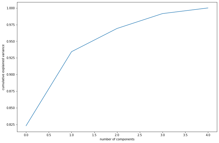
The scree plot can be used to identify the elbow point, which is the point on the plot where the eigenvalues begin to level off. This point represents the number of principal components that should be retained in the data, as the remaining ones do not capture as much variation. They help determine the optimal number of principal components to retain in the data for subsequent analysis, such as data visualization or modeling.

Incremental PCA

Incremental Principal Component Analysis (IPCA) is a variant of Principal Component Analysis (PCA) that allows for calculating principal components on the subset of the data rather than on the entire dataset at once. This is particularly useful when dealing with large datasets too large to fit into memory or requires significant computational resources.

IPCA works by computing the principal components on subsets of the data, called batches, and then incrementally updating the principal components as new data becomes available. The algorithm is designed to minimize the computational cost of calculating the principal components and to ensure that the results are consistent with those obtained using the standard batch PCA algorithm.

The IPCA algorithm can be broken down into the following steps:

1. Initialize the principal components: The first step is to initialize the principal components with arbitrary values. This can be done using a random set of values or the first few samples of the data.

2. Partition of the data into mini-batches: The data is divided into smaller submatrices or mini-batches. The mini-batch size can be chosen based on the available memory and computational resources.

3. Compute the principal components for each mini-batch: The principal components are then computed using the standard PCA algorithm. This involves computing the eigenvectors and eigenvalues of the covariance matrix of the mini-batch.

4. Combine the principal components: The principal components obtained from each mini-batch are combined to obtain the final principal components.

5. Transform the data: Once the final set of principal components is obtained, the data can be transformed into lower-dimensional space using matrix multiplication.

Let us look at an example code shown below.

from sklearn.decomposition import IncrementalPCA
import pandas as pd

a = [[0,0,0],[1,2,3],[2,4,5],[3,6,2],[4,8,3],[5,10,1],[1,2,4],[2,1,5],[3,4,2],[2,8,3],[5,1,1]]
b = ['X','Y','Z']
data = pd.DataFrame(a,columns = b)

ipca = IncrementalPCA(n_components=2, batch_size=6)
ipca.fit_transform(data)

A few changes are made in the code compared to the PCA algorithm. The first and foremost change is that we must mention the batch size here because the algorithm only loads partial data.

In the above example, we let the algorithm automatically divides the data based on the batch size. But we can also fit the IPCA algorithm on smaller batch sizes manually. Refer to the code shown below:

from sklearn.decomposition import IncrementalPCA
import pandas as pd

a = [[0,0,0],[1,2,3],[2,4,5],[3,6,2],[4,8,3],[5,10,1],[1,2,4],[2,1,5],[3,4,2],[2,8,3],[5,1,1]]
b = ['X','Y','Z']
data = pd.DataFrame(a,columns = b)

n = data.shape[0] # Rows we have in the dataset
chunk_size = 5 # Rows we feed to IPCA at a time

ipca = IncrementalPCA(n_components=2, batch_size=6)

for i in range(0, n//chunk_size):
    ipca.partial_fit(data[i*chunk_size : (i+1)*chunk_size])

In the above example, I call the partial_fit function and manually load partial data in chucks.

The most significant advantage of using IPCA is that it can be easily updated as new data becomes available, allowing for real-time analysis and monitoring and more memory-efficient and faster computation.

Use cases of PCA

PCA can be applied to various datasets, including images, audio signals, text, and numerical data. Some typical applications of PCA include:

1. Dimensionality reduction: PCA can reduce the number of features in a dataset while retaining most of the original variation in the data. This can help to speed up computations, reduce memory requirements, and improve the accuracy of machine learning models.

2. Data visualization: High-dimensional data can be challenging in its original form. PCA allows a lower-dimensional data representation to be plotted and explored more easily.

3. Feature extraction: In many cases, the variables in a dataset may be highly correlated. PCA can extract the underlying patterns and relationships in the data by identifying the principal components that capture the most variation.

4. Data compression: By reducing the dimensionality of the data, PCA can also be used for data compression, allowing for more efficient storage and processing of large datasets.

5. Improved model performance: High-dimensional datasets can lead to overfitting and poor model performance. By reducing the dimensionality of the data, PCA can improve the performance of models by reducing the risk of overfitting. It further helps create uncorrelated features/variables that can be an input to a prediction model.

Singular Value Decomposition

Besides the eigenvalue decomposition, singular value decomposition (SVD) is one of the techniques used to calculate the PCA. SVD and Eigendecomposition are matrix factorization techniques that can break down a matrix into constituent parts. However, they differ in terms of the types of matrices they can apply to and their properties.

Eigendecomposition can only be applied to square matrices because if the matrix is not square, it has no inverse. But, SVD can be applied to any m x n matrix, whether square or not. This is the primary difference between the two algorithms.

In eigendecomposition, the matrix X is decomposed to eigenvalues and eigenvectors such that Xv = λv, where v is the eigenvector and λ is an eigenvalue. In SVD, matrix A of dimension n×d is decomposed into a product of three matrices:

$$A = USV^T$$

where, 

• U of dimension n×n and V of dimension n×d are square orthogonal matrices, i.e., \(U^TU=I_d\) and \(V^TV=I_n\)
• S is diagonal (not necessarily square matrix) of singular values having dimension d×n

How is SVD related to PCA?

Let us start with a matrix X that be decomposed using the SVD algorithm as:

$$X = USV^T$$

Let us multiply \(X^T\) on both side of above equation,

$$X^TX = VS^TU^TUSV^T$$

Since we know  \(U^TU=I_d\), therefore, 

$$X^TX = VS^TSV^T$$

\(S^TS\) can be represented as D, as a diagonal with squares of singular values. Therefore,

$$X^TX = VDV^T$$

Moving \(V^T\) on the left side of the equation returns,

$$(X^TX)V = VD$$

which is nothing but the eigendecomposition representation where \(X^TX\) is the matrix, \(V\) is eigenvectors and \(D\) is the eigenvalues.

In summary, while both eigendecomposition and SVD are matrix factorization techniques, they differ in the types of matrices they can apply.

PCA and SVD points to remember

Some important points to remember while using PCA are:

• Most software packages use SVD to compute the components and assume that the data is scaled and centered, so it is essential to do standardization/normalization.
• It should not be used forcefully to reduce dimensionality when the features are not correlated. It works well when features are correlated.
• PCA is limited to linearity, though we can also use non-linear techniques such as t-SNE.
• PCA needs the components to be perpendicular, though that may not be the best solution in some cases. The alternative technique is to use Independent Components Analysis.
• PCA assumes that columns with low variance are not helpful, which might not be accurate in prediction setups (especially classification problems with class imbalance)

Summary

Attaching the notebooks: PCA Explanation that has code snippets used in this blog as a reference. Feel free to download and execute the notebook on your machine for better understanding.

PCA is a dimensionality reduction technique where the primary goal is to generate principal components to choose k < n, i.e., k principal components, and essentially achieve dimensionality reduction, as we eventually want to reduce an m x n dataset with n original features to an m x k dataset with k principal components.

There are two types of decomposition techniques available to find the PCAs. There are eigendecomposition or SVD. Eigendecomposition decomposes the matrix into eigenvalues and eigenvectors such that Xv = λv, where v is the eigenvector and λ is an eigenvalue. In contrast, SVD decomposes the matrix into \(X = USV^T\) where U and V are square orthogonal matrices, and S is the diagonal of singular values.

The article emphasizes the practical applications of PCA and how it can be used for dimensionality reduction, data visualization, feature extraction, data compression, and improved model performance. The post also highlights the importance of standardization or normalization of data before applying PCA and the limitations of PCA, such as linearity and the assumption that columns with low variance are not helpful.

Finally, the article introduces Incremental PCA as a variant of PCA that allows for calculating principal components on the subset of the data rather than on the entire dataset at once.