Part 1: Guide to build accurate Time Series Forecasting models

Time series forecasting is a statistical technique that predicts future values over time based on past observations. Unlike other forms of data analysis, time series forecasting involves analyzing data ordered in time. This means that each observation in the dataset is associated with a specific point in time, such as hourly, daily, weekly, monthly, or yearly.

The primary goal of time series forecasting is to identify patterns in the data and use those patterns to predict future values of the variable being studied. Time series forecasting uses various mathematical and statistical methods discussed in this post to achieve this goal.

One of the critical challenges in time series forecasting is dealing with the unique characteristics of time series data. For example, time series data often exhibit trends, seasonality, and periodicity, making it difficult to identify meaningful patterns in the data. In addition, time series data can be affected by external factors, such as changes in economic conditions or weather patterns, making it difficult to predict future values accurately.

Despite these challenges, time series forecasting remains a powerful tool for businesses and organizations that rely on data to make decisions. Organizations can optimize their operations, reduce costs, and stay ahead of the competition by identifying patterns in time series data and making accurate predictions about future values.

Time series forecasting is a critical technique used in industry. But how is it different from the machine learning regression techniques?

How is the time series forecast different from the regression?

This is the most general question when encountering the time series problem and seeing that we need to predict the target variable is continuous. We may think we can use regression or advanced regression to make a forecast, taking time as an independent variable. However, this will not work due to various reasons. One reason is that in a time series, the sequence is essential.

If we shuffle the dataset, the results we will get from the regression problem will be similar, but in the case of the time series forecast, the result will be different.

Why does this happen? This happens because while forecasting using time series, your model predicts not only based on the values given but also on the sequence in which the values are given. Hence, the sequence is crucial in a time series analysis and should not be played around.

Therefore, it's safe to state that time series have a solid temporal (time-based) dependence. Each data set consists of a series of timestamped observations, i.e., each observation is tied to a specific time instance. Thus, unlike regression, the order of the data is essential in a time series.

Further, in a time series, we are unconcerned with the causal relationship between the response and explanatory variables. The cause behind the changes in the response variable is a black box.

Let us understand this with the help of an example. We want to predict the stock market index's value next month. We will not look at why the stock market index increases in value if it's because of an increase in GDP or if there are some changes in any sector or other factor. We will only look at the sequence of values for the past months and predict the next month based on that sequence.

NOTE: Though techniques are available to include such regressors variables in time series analysis. We will be covering them in upcoming posts.

Let us start our post by understanding the different forecasting types involved in time series forecasting.

Different types of forecasting

Qualitative and quantitative forecasting are two broad categories of time series forecasting methods that differ in their approach to predicting future values.

Qualitative Forecasting

Qualitative forecasting methods rely on expert judgment and subjective assessments of future trends and conditions. These methods are helpful when historical data is unavailable or unreliable or when significant environmental changes make it difficult to use past data to predict future values. Examples of qualitative forecasting methods include market research, surveys, and the Delphi method.

Quantitative Forecasting

Quantitative forecasting methods, on the other hand, rely on historical data and statistical models to make predictions about future values. These methods are based on the assumption that past trends and patterns can be used to predict future behavior. Examples of quantitative forecasting methods include time series analysis or artificial neural networks.

The choice of forecasting method depends on several factors, including the availability and quality of historical data, the level of uncertainty and complexity in the environment, and the expertise and resources of the forecaster. In some cases, a combination of qualitative and quantitative forecasting methods may be used to improve the accuracy and reliability of the forecast.

The process to solve the time series forecasting problem

In this blog, we will be discussing quantitative forecasting methods only. Before starting, let's dive into the terminology used throughout this post.

• Time Series Data: Any data with a time component could be termed time-series data. For example, the number of orders made on a food ordering app per day is an example of time series data.
   
• Time Series Analysis: Performing analysis on time series data to find valuable insights and patterns is termed time series analysis.
   
• Time Series Forecasting: Time series forecasting looks at past data to predict the future. E.g., the food ordering app wants to predict the number of orders per day for the next month to plan the resources better.

Like any traditional machine learning problem-solving approach, we start with defining the problem, data collection, analyzing the data, and handling missing values and outliers. Finally, we build and evaluate the forecast model. But massaging the data and fitting a time series algorithm differs. Let's understand the process involved in the time series in detail.

1. Defining the problem

Defining the problem is the first step in the pipeline. Here we define our goal and answer the question: 'What to forecast?'. It involves identifying the issue or challenge that needs to be addressed, clarifying the scope and nature of the problem, and establishing clear goals and objectives for solving the problem.

We pay attention to the following details while defining the problem.

• Quantity: This specifies what quantity we are forecasting. E.g., number of passengers or units sold.
• Granularity: Depth at which we are forecasting for. E.g., Single store, retail, warehouse, etc.
• Frequency: Duration of forecasting. E.g., Weekly, Monthly, Yearly, etc.
• Horizon: Short-term, mid-term, or long-term forecast. E.g., one year (12 months)

There is a rule of thumb that should be kept in mind when we are solving time series problems:

The Granularity Rule

The more aggregate your forecasts, the more accurate you are in your predictions simply because aggregated data has lesser variance and noise.

Let's understand this with the help of an example. Suppose I work as a country head and want to predict the sales for a few newly launched products for the following year. Would I be more accurate in my predictions if I predicted at the city or store levels? Accurately predicting the sales from each store might be difficult.

Still, when I sum up the sales for each store and present my final predictions at a city level, my predictions might be surprisingly accurate. This is because, for some stores, I might have predicted lower sales than the actual ones, whereas the sales might be higher for some. And when I sum all of these up, the noise and variance cancel each other out, leaving me with a good prediction. Hence, it would help if I did not make predictions at very granular levels.

The Frequency Rule

This rule states to keep updating forecasts regularly to capture any new information that comes in.

Let's continue with an example of forecasting product sales to understand this rule. Say my frequency for updating the forecasts is three months. Due to the COVID-19 pandemic, the residents may be locked in their homes for around 2-3 months, during which the sales would have dropped significantly. Now, if the frequency of my forecast is only three months, I cannot capture the decline in sales, which may incur significant losses and lead to mismanagement.

The Horizon Rule

When I have the horizon planned for many months into the future, I am more likely to be accurate in the earlier months than the later ones.

Let's again go back to the example of forecasting product sales to understand this rule. Suppose I predicted the sales for the next six months in March 2023. It may have been entirely accurate for the first two months. Still, due to the unforeseen COVID-19, the sales in the next few months would have been significantly lower than predicted because everyone stayed home. The farther ahead we go into the future, the more uncertain we are about the forecasts.

2. Data Collection

Data collection is a critical step in time series forecasting, as the accuracy and reliability of the forecast depend on the quality and quantity of the data used. There are three essential characteristics that every time series data must exhibit for us to make a good forecast.

1. Relevant: The time series data should be relevant to the objective we want to achieve.
2. Accurate: The data should accurately capture the timestamps and observations.
3. Long enough: The data should be long enough to forecast. This is because it is essential to identify all the patterns in the past and forecast which patterns will repeat in the future.

Data collection requires careful planning, execution, and validation to ensure the accuracy and reliability of the forecast. It is a famous saying goes, "Garbage In, Garbage Out."

3. Analyzing the Data

Analyzing data in time series forecasting provides insights into the underlying patterns and trends that can be used to develop accurate predictions. While analyzing the data, there is a different component of the time series that needs to be focussed upon, as discussed below:

• Level: The level component represents the time series' overall average or baseline value. It is the average value of the series over time, assuming there is no trend, seasonality, or cyclicity. It is a static component that doesn't change over time.
   
• Trend: The trend component represents the time series' long-term upward or downward movement. It shows the overall direction of the series over time. A trend can be linear or non-linear, and it can be positive or negative.
   
• Seasonality: The seasonality component represents the repetitive pattern or cycle of the time series that occurs within a year or a specific period. For example, sales of winter clothing may have a seasonal pattern that peaks in the winter months and drops in the summer months. Seasonality is a regular pattern that repeats itself over time.
   
• Residuals: Residual is the part left over after extracting trend and seasonality from the time series.
   
• Cyclicity: The cyclicity component represents the periodic patterns or cycles of the time series that occur over a more extended period than seasonality. Cyclicity is less regular than seasonality and can last for several years. Examples of cyclical patterns include business cycles, which refer to the periodic expansion and contraction of the economy.
   
• Noise: The noise component represents the random fluctuations or irregularities in the time series that cannot be attributed to the other components. Noise is the variation in the data that is not explained by the level, trend, seasonality, or cyclicity. Noise is a random and unpredictable component.

Understanding these components is vital for analyzing and modeling time series data. By identifying and separating these components, analysts can better understand the underlying patterns and trends in the data and develop more accurate models for forecasting and prediction.

4. Handling Missing Values

It's common for datasets to have missing values for multiple reasons. It may be that operations are closed, data entry issues, systematic reasons, or malfunctioning happening. There are some common strategies to impute missing values in time series data:

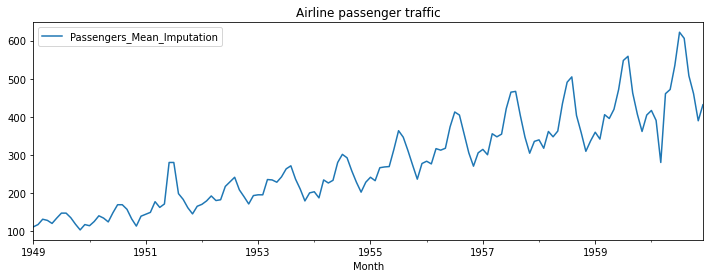
• Mean Imputation: Imputing the missing values with the overall mean of the data. This is the most common way to use in machine learning problems. Imputing the missing value with mean, median, and mode can reduce the variance, and the trend may be missed if we use mean imputers.
   
• Last observation carried forward: We can attribute the missing values to their previous value in the data. Imputing the missing value with the next observed value and last observed value can introduce bias in analysis and perform poorly when data has a visible trend.
   
• Linear interpolation: You draw a straight line joining the data's next and previous points of the missing values. This method captures trends quite well but doesn't capture seasonality.
   
• Seasonal + Linear interpolation: This method best applies to the data with trend and seasonality. Here, the missing value is imputed with the average of the corresponding data point in the previous seasonal period and the following seasonal period of the missing value.

Overall, the choice of approach for handling missing values in time series data depends on the characteristics of the data and the nature of the missing values. Further, analysts should carefully document any missing value treatment that is applied, as this can affect the accuracy and reliability of the forecasting model.

5. Handling Outliers

Outliers are extreme data points in the dataset that can occur due to extreme conditions or demand, which never occurs again, errors in data entry, etc. Below are a few of the methods and techniques that are commonly used to detect outliers:

• Extreme value analysis: The analysis involves finding the smallest and largest values in the dataset.
   
• Box Plot: The points on either side of the whiskers are considered outliers. The length of these whiskers is subjective and can be defined by you according to the problem.
   
• Histogram: Simply plotting a histogram can also reveal the outliers - the extreme values with low frequencies visible in the plot.

Using the above techniques, one can perform an analysis of the outliers. To remove the outliers from the dataset below techniques can be used:

• Trimming: Technique of simply removing the outliers. It may be subjective to the use case we are trying to solve.
   
• Lower and upper capping: Decide the lowest and upper band; any data point that occurs beyond is replaced with the respective band.
   
• Zero capping: Cases where the value cannot be negative such as sales, account balance, etc. In such cases technique of zero capping is used.

It's essential to carefully consider the nature and cause of the outliers when choosing a method for handling them, as different methods may be more effective in different situations.

6. Build and evaluate the forecast model

Before building the model, we decompose the dataset into trend, seasonality, and residuals. Let's assume we have a dataset for airline passenger traffic that states the monthly number of passengers traveling by air.

And we want to find the decomposition of the dataset. There are two ways in which the time series data can be decomposed:

Additive Seasonal Decomposition 

Additive Seasonal Decomposition assumes that the seasonal component is constant throughout the time series and is added to the trend and irregular components. The decomposition formula for an additive model is:

y = T + S + I

where y is the observed data, T is the trend, S is the seasonal component, and I is the irregular component.

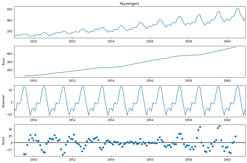
The above diagram states the additive decomposition of the airline passenger dataset discussed above.

In an additive model, the seasonal component is constant and does not change over time. For example, if the seasonal component is 10, it is added to every observation in the time series to account for the seasonal pattern. An additive model is appropriate when the magnitude of the seasonal component does not vary with the level of the series.

Multiplicative Seasonal Decomposition

Multiplicative seasonal decomposition assumes that the seasonal component is proportional to the time series level and is multiplied by the trend and irregular components. The decomposition formula for a multiplicative model is:

y = T * S * I

where y is the observed data, T is the trend, S is the seasonal component, and I is the irregular component.

In a multiplicative model, the seasonal component varies proportionally with the level of the series. For example, if the seasonal component is 10 and the series level is 100, then the seasonal component is 10% of the series level. A multiplicative model is appropriate when the seasonal component's magnitude varies with the series' level.

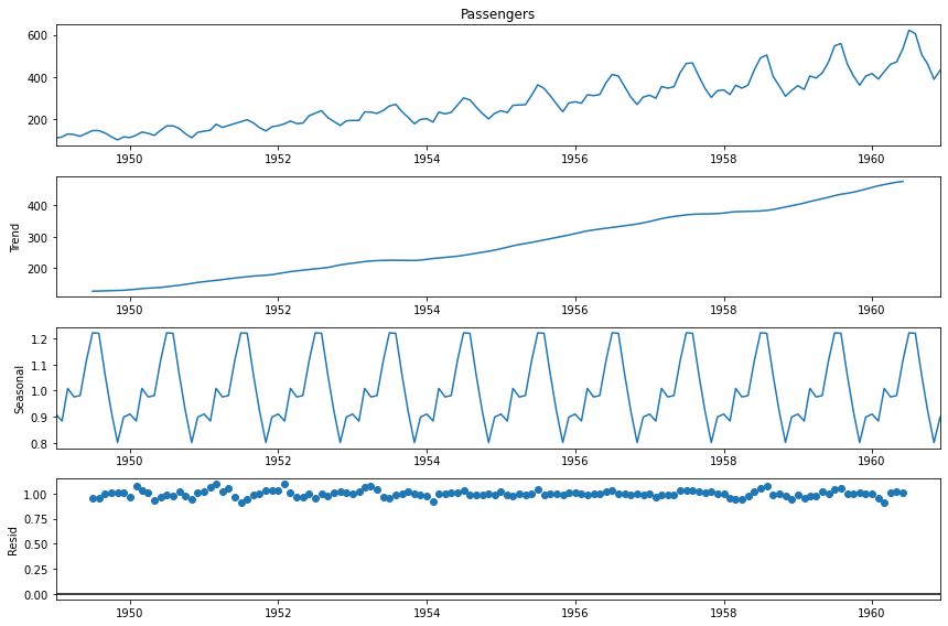
The above diagram states the multiplicative decomposition of the airline passenger dataset discussed above.

After decomposing the dataset into trend, seasonality, and residuals, the next step is to build a model that can forecast. Many methods are available to build and evaluate time series models. We will look at such techniques in the remaining section of the post.

Basic Forecasting Methods

Forecasting is the process of making predictions about future events based on past and present data. Basic forecasting methods are simple and commonly used methods for making forecasts.

These methods can be applied to a wide range of data and do not require advanced statistical knowledge or software. Basic methods include naive forecasting, moving averages, exponential smoothing, and trend projection. These methods help provide a quick and straightforward forecast, but they may not always be accurate or suitable for more complex data.

Understanding these basic methods is essential for anyone who needs to make forecasts in their work or personal life, such as business owners, financial analysts, and economists. Let's get started.

Naive Method

The naive method is one of the simplest and most commonly used forecasting methods. It is a forecasting method that assumes that the future value of a time series will be the same as the current value.

This means that the naive method predicts that the future will be the same as the present and that there will be no trend, seasonality, or other underlying patterns in the data.

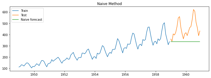
The example shown above represents the passengers traveling by air monthly. In the graph, the blue line indicates the training dataset, the orange line indicates the actual value of the test dataset, and the green line indicates the forecasted value from the algorithm. We will use the same color code for the rest of the post. As we can see, using the Naive method, the last value observed in the time series is forecasted for all future periods.

Simple average method

The simple average method is a primary forecasting method that uses the average of past observations to predict future values. This method assumes that the future values of a time series will be similar to the average of past values.

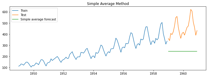
In the example shown above, the green line, which represents the forecasted value, is the sales average across the month of the training data.

Simple moving average

What if we take only the last few sets of observations to predict the future, as the last observation has more impact on the future than the first observation? This is where the simple moving average comes into the picture.

It is a popular forecasting method similar to the simple average method but forecasts better than it. Considering that the last observation in the time series has more impact on the future rather than the first observation, in the simple moving average method, we take the average of only the last few observations to forecast the future.

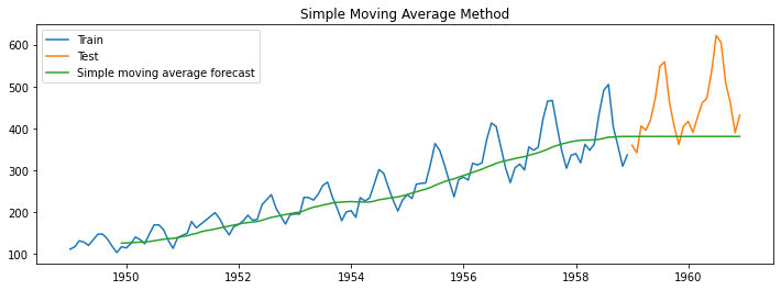
Choosing a window of moving average is always a tradeoff between the trend cycle pattern and how much noise we allow. The shorter the moving average window, the higher the trend we capture and the more noise we allow in the forecast. In the example shown above, the forecasting is done with a window size of 12. Do you think it is the right choice for the window size? Post your thoughts in the comment section below.

Simple Exponential Smoothing

This technique uses a weighted average of past observations to predict future values. In the simple moving average technique, we consider each observation in that window to equally influence the next value in the forecast. But intuitively, the most recent observations influence the next value more than past observations.

The weighted moving average technique is that each observation influencing \(y_{t+1}\) is assigned a specific weight. More recent observations get more weight, whereas the previous observations get less weight.

Simple Exponential Smoothing captures the level component of time series data. In this smoothing technique, the forecast observation data, \(y_{t+1}\), is a function of the level component denoted by \(I_{t}\). Here, the level component is written as follows:

$$l_t = \alpha.y_t + (1- \alpha).l_{t-1}$$

The most recent value \(y_t\) takes a weight of α, also known as the level smoothing parameter, whereas the previous observation's level component takes the value of 1−α. The values of α lie between 0 and 1.

On replacing the value of the \(l_t\), \(y_{t-1}\), \(y_{t-2}\), . . . and so on, we will get the below equation:

$$\hat{y}_{t+1} = \alpha.y_t + \alpha.(1- \alpha)y_{t-1} + \alpha.(1- \alpha)^2y_{t-1}....$$

Since the value of the weight assigned to every observation decreases exponentially, this technique is called an exponential smoothing technique.

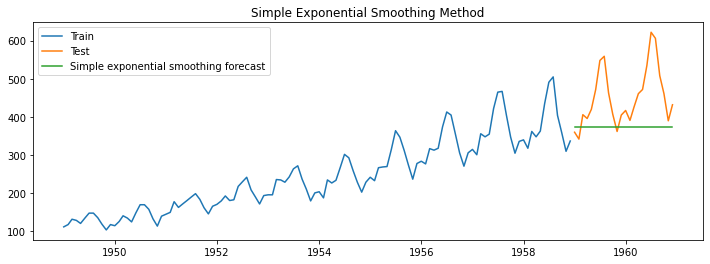
In the example shown above, the alpha value is set to 0.2. We are successfully able to capture the level of the time series data. We are not able to capture the trend and seasonality of the passengers traveling by air monthly.

Holt's Exponential Smoothing

As we have discussed above, the simple exponential model captures the level of a time series. Holt's exponential smoothing technique captures the forecast's level and trend of a time series. Holt's exponential smoothing is particularly useful for data sets with a trend that changes over time, as it allows the forecast to adjust for trends.

The forecast equation for holt's exponential smoothing is a function of both level and trend; that is, 

$$\hat{y}_{t+1} = l_t + b_t$$

Here \(l_t\) is the level component, and \(b_t\) is the trend component.

Here, the trend component is calculated as follows: 

$$\hat{b}_{t} = \beta(l_t - l_{t-1}) + (1 - \beta)b_{t-1}$$

Here β is the smoothing parameter for the trend.

The equation for the level component remains the same as discussed in Simple Exponential Smoothing with the minor addition of the previous value's trend component in calculating the previous value's level component.

$$l_t = \alpha.y_t + (1- \alpha).(l_{t-1} + b_{t-1})$$

The higher value of β better the capability to capture the short-term trend or more recent trend, and the lower the β value better the capability to capture the long-term trend. Therefore we strive to find the balance between the β values. Let us again consider our air passenger traffic example.

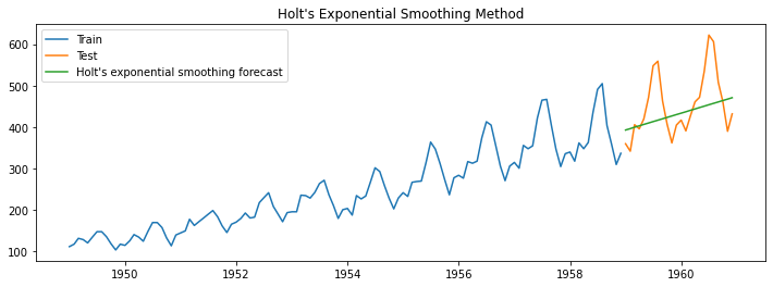
For the example shown above, we consider the alpha value 0.2 and the beta value 0.01, representing level and trends, respectively. This time we observed that both level and trend are captured for the given time series example. But the seasonality component is still not captured. Let us look at Holt-Winters's Exponential Smoothing, which can help capture the seasonality component, level, and trend.

Holt-Winters's Exponential Smoothing

The basic idea behind Holt-Winters' exponential smoothing is to decompose the time series into three components: level, trend, and seasonality. The method uses three smoothing factors: α (for the level), β (for the trend), and γ (for the seasonality).

The α parameter controls the weight given to the most recent observation in the level estimate, while the β parameter controls the weight given to the most recent trend estimate. The γ parameter controls the weight given to the most recent seasonal estimate. The forecast equation now has seasonal components, including level and trend i.e.

$$\hat{y}_{t+1} = l_t + b_t + S_{t+1-m}$$

Here, m is the number of times a season repeats during a period. The seasonal component is calculated using the following equation:

$$S_t = \gamma.(y_t - l_{t-1} - b_{t-1}) + (1 - \gamma).s_{t-m}$$

Where γ is the weight assigned to the seasonal component of the recent observations.

The trend and the level equations, respectively, are as follows:

$$\hat{b}_{t} = \beta(l_t - l_{t-1}) + (1 - \beta)b_{t-1}$$

$$l_t = \alpha.(y_t - s_{t-m})+ (1- \alpha).(l_{t-1} + b_{t-1})$$

There are two methods of performing the Holt-Winters' smoothing techniques: additive and multiplicative.

In the additive method, the seasonal variation is added to the level and trend estimates. The multiplicative method multiplies the seasonal variation by the level and trend estimates. The appropriate method depends on the data's nature and the seasonality pattern.

But generally speaking, the additive method is more appropriate when the seasonal variations are roughly constant over time, and the magnitude of the seasonal variation does not change with the level of the time series. This means that the size of the seasonal variation is independent of the level of the time series.

On the other hand, the multiplicative method is more suitable when the seasonal variations are proportional to the level of the time series. This means that the size of the seasonal variation changes as the level of the time series changes.

One of Holt-Winters' exponential smoothing strengths is its ability to handle data sets with complex seasonal patterns. However, it is essential to note that this method may not be suitable for all types of time series data. Additionally, Holt-Winters' exponential smoothing requires significant historical data to accurately estimate the three smoothing parameters.

Let us again consider our example of airline passenger traffic and apply the multiplicative method of Holt-Winters' exponential smoothing.

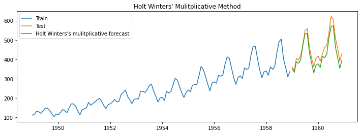
We observe that the method has worked well. All three components of level, trend, and seasonality are captured well, as the difference between the forecasted green and orange test dataset lines is minimal. We will understand how to measure the time series model's performance in the next section of this post.

Measuring Model Performance

Error measure that we use to calculate the model's error during the forecast.

Mean Forecast Error (MFE)

In this naive method, we subtract the actual values of the dependent variable, i.e., 'y', with the forecasted values of 'y'. This can be represented using the equation below.

$$MFE= {1\over n} \sum^n_{i=1}(y_{actual} - \hat{y}_{forecast})$$

Mean Absolute Error (MAE)

Since MFE might cancel out a lot of overestimated and underestimated forecasts, measuring the mean absolute error or MAE makes more sense as, in this method, we take the absolute values of the difference between the actual and forecasted values.

$$MAE= {1\over n} \sum^n_{i=1}|y_{actual} - \hat{y}_{forecast}|$$

Mean Absolute Percentage Error (MAPE)

The problem with MAE is that even if we get an error value, we have nothing to compare it against. For example, if the MAE you get is 1.5, we cannot tell, based on this number, whether you have made a good forecast.

Suppose the actual values are in single digits. In that case, the MAE error is 10.5, which is high. But then the actual values are in the order of thousands. In that case, an error of 10.5 indicates a good forecast.

To capture how the forecast is doing based on the actual values, we evaluate the mean absolute error, where we take the mean absolute error (MAE) as the percentage of the actual values of 'y'.

$$MAPE= {100\over n} \sum^n_{i=1}|{{y_{i} - \hat{y}_{i}} \over y_i}|$$

Mean Squared Error (MSE)

The idea behind the mean squared error is the same as the mean absolute error. But this time, we want to capture the absolute deviations so that the negative and positive deviations do not cancel each other out. To achieve this, we square the error values, sum them up and take their average. This is known as mean squared error or MSE, which can be represented using the equation below.

$$MSE= {1\over n} \sum^n_{i=1}(y_{actual} - \hat{y}_{forecast})^2$$

Root Mean Squared Error (RMSE)

Since the error term we get from MSE is not in the same dimension as the target variable 'y' (it is squared), we use a metric known as RMSE wherein we take the square root of the MSE value obtained.

$$RMSE= \sqrt{{1\over n} \sum^n_{i=1}(y_{actual} - \hat{y}_{forecast})^2}$$

Several performance measures can be used to evaluate the accuracy of time series models. The above-stated are a few popular methods that are considered to measure the performance of the time series models and build accurate time series forecasting models. It's essential to choose the appropriate measure based on the nature of the data and the forecasting goals. Additionally, it's recommended to use multiple measures to get a more comprehensive understanding of the model's performance.

Bonus Tip

If you have experience working on traditional machine learning problems, you would have come across the concept of cross-validation. It is a machine learning technique to evaluate a model's performance on an independent dataset. The concept behind cross-validation is to divide the available data into two sets: a training set, which is used to train the model, and a validation set, which is used to evaluate the model's performance.

The most common method of cross-validation is k-fold cross-validation. In k-fold cross-validation, the available data is divided into k subsets of equal size. The model is trained on k-1 of these subsets and evaluated on the remaining subset. This process is repeated k times, with each subset used as the validation set precisely once. The performance measures obtained from each fold are then averaged to estimate the model's overall performance.

But applying cross-validation to time series data can be a bit more challenging than other data types, as the data is inherently ordered and observations depend on previous observations.

Let's understand the two validation types that can help apply cross-validation techniques to time series data.

One-Step Validation

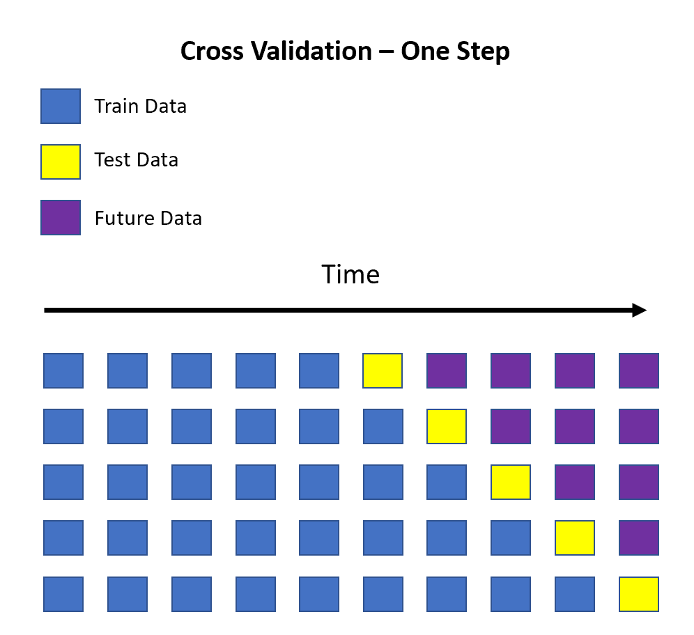
One-step cross-validation is a technique used in time series forecasting to evaluate the performance of a model by comparing its predicted values to the actual values in the validation set. It involves using a fixed-size historical dataset to train the model and then using the following observation as the validation set to assess the accuracy of the model's predictions.

For example, let's say we have a time series with 10 observations, and we want to evaluate the performance of a model using one-step cross-validation. We could start by training the model on the first 5 observations and then using the 6th observation as the validation set. We would then calculate the error between the predicted and actual values for the 6th observation. This process is then repeated for the remaining observations.

This idea is represented in the image below. Here the blue squares represent the train data, the yellow squares represent the test data, and the purple ones are the future values for which the initial test points must be predicted first. In the image below, we have 6 test data points; hence it takes six iterations (or forecasts) to predict the test set fully.

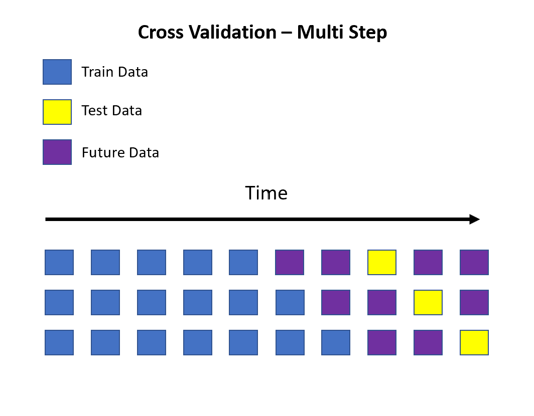
Multi-Step Validation

This is the same as one-step validation; the only difference is that we do not consider a few points to the immediate right of the last training data point but rather skip a few points to make forecasts well into the future. This can be seen in the image below.

Conclusion

I have created a jupyter notebook in the git repo for reference for all the time series forecast models trained above. Feel free to use it as a guide and perform hands-on to understand the concept better. I firmly believe that we can only learn and, most importantly, remember if we can do hands-on.

This post provides an overview of building and evaluating time series forecasting models. The steps include data preparation, exploratory data analysis, handling outliers, building and evaluating the forecast model, and measuring model performance.

Basic forecasting methods such as naive forecasting, moving averages, exponential smoothing, and trend projection are also discussed. The post also explains how to decompose a time series into trend, seasonality, and residuals using additive and multiplicative seasonal decomposition methods.

Finally, various error measures such as mean forecast error, mean absolute error, mean absolute percentage error, mean squared error, and root mean squared error is explained to evaluate the accuracy of time series models.

To learn more about AR based models, refer to the post Part 2: Guide to build accurate Time Series Forecasting models - Auto Regressive Models.