Naïve Bayes Algorithm Detailed Explanation

In this post, I will be talking about the Naïve Bayes algorithm which is a popular machine learning algorithm used for text-based tasks. Naïve Bayes is a probabilistic classifier that returns the probability of a test point belonging to a class rather than the label of the test point.

It is a bayesian method that combines evidence from data (summarized by the likelihood) with initial beliefs (known as a prior distribution) to produce a posterior probability distribution of the unknown quantity. We will be demystifying the above statement in this post.

The classifier finds a good use case in text-based tasks such as classifying emails into spam or ham. Before we deep dive into the understanding of the Naïve Bayes algorithm, let us first understand the conditional probability and Bayes theorem which is the prerequisites. 

Conditional Probability

As we know the probability of event E is defined as:

P(E) = Number of favorable outcomes / Total number of possible outcomes

In the same way, conditional probabilities are nothing but the probability of an event given some event has already occurred. Or in other terms, conditional probability is defined as the likelihood that an event will occur, based on the occurrence of a previous outcome. Let's take an example to understand conditional probability.

Assume, we are given a task to build an email spam classifier and we want to classify an email as spam or not. Let us further simplify, I am given that the email contains the word "FLAT DISCOUNT" and now I want to classify the email as SPAM or HAM.

Or in other terms P(SPAM | word= "FLAT DISCOUNT") will be high or low? For me, it is definitely going to be very high. What do you think?

A few other examples where conditional probabilities are used in real-world are:

• Every time Dhoni hits a half-century, there are 70% chances India won.
• Given that it is a rainy day, the probability of having 60% of employees in the office will be 20%.

Conditional probability is needed to understand relative probabilities, which is more often the case in real-world scenarios instead of looking into the absolute probability of events in isolation.

Let us define two terms prior probabilities and posterior probabilities before we proceed forward.

Let us consider our example of an email classifier again. The probability of an email being spam is the prior probability with no other information given. Let's say based on historical data probability of an email being spam is 5%. Therefore this is the prior probability.

And posterior probability on other hand is the probability given the fact that some other event has occurred. In our example of an email classifier, the probability of an email being spam given an email having the word "FLAT DISCOUNT" or P(SPAM | word= "FLAT DISCOUNT") is called posterior probability.

NOTE: Posterior probability is a special case of conditional probability, where the condition is explicitly the evidence from an experiment being used as the condition.

Having an understanding of prior and posterior probabilities as well as conditional probability, let us proceed forward and understand what is Bayes theorem.

Bayes Theorem

Bayes Theorem is a mathematical formula used to determine a given event's conditional probability. Let us take an example and understand how Bayes Theorem can be used for calculating conditional probabilities.

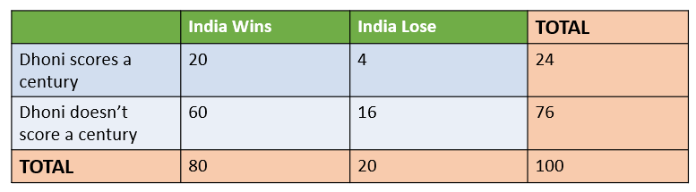
Consider an example where the historical cricket data is considered and data is provided when India wins or losses the match when Dhoni scores a century or doesn't score a century.

Let us calculate the probability that India wins, given that Dhoni has scored a century. There are a few probabilities that we need to calculate first before answering this question.

You can pause here and try to calculate the answer to the above question and compare it with the answer calculated later in this post.

Joint Probability

A joint probability is a statistical measure that is used to calculate the probability of two events occurring together at the same point in time and is represented as P(A, B) or \(P(A \cap B)\) where,

$$P(A, B) = { P(A) * P(B) }$$

, given that A and B are independent events.

Let us take the above example again and calculate the joint probability of India winning the match AND Dhoni scoring a century. Intuitively, looking at the table we can see that 20 times Dhoni has scored a century and India has won the match out of 100.

Therefore, intuitively speaking the probability of India winning the match AND Dhoni scoring a century should be 20 / 100 or 2%. Let us drive this using joint probability.

Mathematically, the joint probability is the interaction of two events A and B and is calculated as the multiplication of P(A) and P(B).

P(A = India Win) = 80 / 100 and P(B = Dhoni scores century) = 24 / 100

NOTE: Here A and B events are not independent events therefore P (A) * P(B) will not be applicable. 

Therefore, (P(A \cap B)\) can be calculated as P( B| A) * P(A) = 20/80 * 80/100 = 20/100, which is the same as per the calculation we have done intuitively.

NOTE:  \(P(A \cap B)\) = \(P(B \cap A)\)

So how are joint probability and conditional probability different from one another?

In joint probability, the total sample space does not get affected (remains 100) whereas in conditional probability the total sample space gets reduced to the number of times the event we are conditioning on occurs (changes to 24. Number of times when Dhoni scores a century)

Calculating Bayes Theorem

As per Bayes theorem, 

$$P(A | B) = { P(B|A) . P(A) \over P(B)}$$

Or can be rewritten as,

$$P(A | B) = { P(A \cap B)\over P(B)}$$

Or we can also rewrite the above equation as,

$$P(A \cap B) = { P(A|B) . P(B)} = { P(B|A) . P(A)}$$

\(P(A \cap B)\) = 10/12 * 12/ 100 = 10/100, which is the same as calculated using the formula \(P(A \cap B)\) = P(A) * P(B).

Now, we are well equipped with the information needed to understand how the Naïve Bayes algorithm works.

Naïve Bayes Algorithm

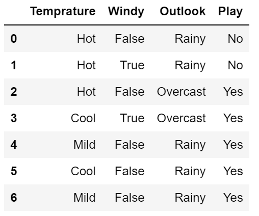
Let's say we have features that are categorical (Temperature, Windy, and Outlook) in nature and we need to predict the target class (Play) which is binary in nature. The Naïve Bayes algorithm uses Bayes’ theorem to classify new test points. Consider we have the dataset as shown below:

Recall from Bayes Theorem,

$$P(C_i | x) = { P(x | C_i) .P(C_i)\over P(x)}$$

where \(C_i\) denotes the classes in the dataset and \(x\) denotes the features in the dataset. Let's apply this formula only to one independent variable Temperature.

$$P(C=Play | x=Hot) = { P(x=Hot | C=Play) .P(C=Play)\over P(x=Hot)}$$

$$P(C=Don't Play | x=Hot) = { P(x=Hot | C=Don't Play) .P(C=Don't Play)\over P(x=Hot)}$$

NOTE: The denominator is common among both of the equations and therefore can be ignored as we will be comparing and classifying data points into one of two classes.

So far we are able to solve the problem when we have one feature available in the dataset. But, how do we solve the problem when there is more than one feature in the dataset which is generally the case?

Multivariate Naïve Bayes classification

Let us again consider our previous example and this time let's add another column "Windy". Now we have two independent variables (Temperature and Windy) and one dependent variable (play or not). Let's see how to apply Bayes's theorem in such a scenario.

We need to calculate,

$$P(C=Play | x=(Hot, False)) = { P(X = Hot, False | C= Play).P(C=Play)\over P(x=Hot, False)}$$

Assuming cap surface and cap shape are the independent variables. Therefore, \(P(X = Hot, False | C= Play)\) can be written as \(P(X=Hot | C=Play) .(X=False | C=Play)\). Therefore above equation can be written as:

$$P(C=Play | x=(Hot, False)) = { P(x=Hot | C=Play).P(x=False | C=Play) .P(C=Play)\over P(x=Hot, False)}$$

Now the individual probabilities can be calculated from the dataset.

$$P(C=Play | x=(Hot, False)) = { 1/7 * 4/7 * 5/7 \over P(x=Hot, False)}$$

And the probability that the mushroom is poisonous or not. 

$$P(C=Don't Play | x=(Hot, False)) = { P(x=Hot | C=Don't Play).P(x=False | C=Don't Play) .P(C=Don't Play)\over P(x=Hot, False)}$$

$$P(C=Don't Play | x=(Hot, False)) = { 2/7 * 1/7 * 2/7 \over P(x=Convex, Smooth)}$$

Since we are comparing, therefore, the denominator can be excluded. \(P(C=Play | x=(Hot, False))\) is greater than the \(P(C=Don't Play | x=(Hot, False))\) therefore we classify the datapoint that we can go ahead and play.

This is how conditional independence helps in calculating the class probabilities in the case of a dataset having more than one feature. In the same way, the concept can be extended to more than two variables as well as shown below:

$$P(C=Play | x) = { P(x | C=Play) .P(C=Play)\over P(x)}$$

where x represents different variables.

Now \(P(x | C=Play)\)  can be broken down into as many variables probabilities considering conditional independence as shown below:

$$P(x | C=Play) = P(x_1 | C=Play).P(x_2 | C=Play).P(x_3 | C=Play).P(x_4 | C=Play) . .. . P(x_n | C=Play)$$

In this way, we can calculate the multivariate Naïve Bayes probabilities.

Calculating Naïve Bayes for continuous variables

In the examples shown above, we have calculated the Naïve Bayes algorithm specifically for the categorical data and this is where the Naïve Bayes algorithm finds most of its use cases. But the algorithm can also be extended to continuous data as well.

For continuous data, the mean and standard deviation are considered assuming the variable follows a normal distribution, and then using some Z-table the probabilities can be calculated for each continuous variable. And then the calculated probabilities can be plugged into the naive Bayes algorithm.