Logistic Regression Detailed Explanation

Logistic regression is a binary classification model, i.e. it will help to make predictions in cases where the output is a categorical variable.

We cannot draw a line and classify data points into two classes. So we can use the curve also known as the sigmoid curve. The sigmoid function is represented as:

$$ 1\over {1 + e^{-(\beta_0 + \beta_1x)}}$$

As we know Linear Regression is represented as:

$$h_\theta(x) = w^Tx$$

and the Logistic regression is represented as \(h_\theta(x) = g(w^Tx)\),  where we can represent \(z\) = \(w^Tx\). Therefore \(g(z)\) is represented as:

$$g(z) = {1 \over {1+e^{-z}}}$$

The above function which is known as sigmoid function or logistic function is graphically represented as shown below:

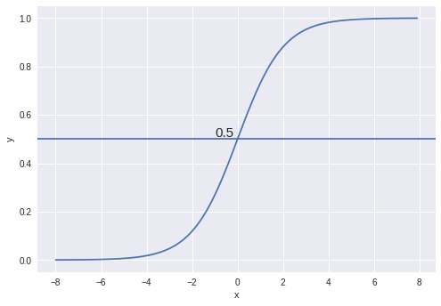
Properties of the sigmoid curve are:

1. It has extremely low values at the start.
2. It has extremely high values in the end.
3. It has intermediate values in the middle.

Are you wondering why can't we fit the straight line and we fit a sigmoid function or Logistic function? The reason why we can’t use a straight line or Linear Regression is as follows:

• The straight line is not steep enough. In the sigmoid curve, we have low values for a lot of points, then the values rise all of a sudden, after which you have a lot of high values.
• In Linear regression, the output can be much larger than 1 or significantly smaller than 0 for the classification problem where we just need 0 or 1 as the output.
• In a straight line, the values rise from low to high very uniformly, and hence, the boundary region (the one where the probabilities transition from low to high) is not present.

Because of the above-mentioned reasons, we need different algorithms for classification problem and we can't use Linear Regression.

NOTE: The logistic regression model separates two different classes using a line linearly. The sigmoid curve is only used to calculate class probabilities. The final classes are predicted based on the cutoff chosen after building the model.

Best Fit for Sigmoid Curve

As we have seen in the sigmoid function, there is β0 and β1 which we need to find for the best fit. The best fit sigmoid curve would be the one that maximizes the value of the product shown below.

Consider an example where we have a few points that belong to class 1 or 0. Refer to the diagram shown below:

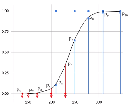
Our goal is to find the sigmoid curve such that \((1-P_1)(1-P_2)(1-P_3)(1-P_4)(1-P_6)(P_5)(P_7)(P_8)(P_9)(P_10)\) is maximized. This product is called the likelihood function.

To find β0 and β1 for the best fitting sigmoid curve, we would have to try a lot of combinations, unless we arrive at the one which maximizes the likelihood.

Doesn't this sound similar to the linear regression problem? Where we find β0 and β1 until we have the combination that minimizes the cost function.

Now, the next huddle is to find optimize the value of β0 and β1. The optimization method used to find β0 and β1 is the Maximum Likelihood Estimation (MLE).

Maximum Likelihood Estimation (MLE)

Unlike the linear regression model, that uses Ordinary Least Square for parameter estimation, we use the Maximum Likelihood Estimation for Logistic Regression.

MLE is basically a technique to find the parameters that maximize the likelihood of observing the data points assuming they were generated through a given distribution like Normal, Bernoulli Distribution, etc. Before directly jumping to MLE for the logistic regression we will first look at the MLE for continuous and discrete distributions.

• Maximum Likelihood Cost Function
• Maximum Likelihood Estimation for a continuous distribution
• Maximum Likelihood Estimation for a discrete distribution
• Maximum Likelihood Estimation for a logistic function
• Estimating the parameters via Iterative techniques
  • Gradient Descent
  • Newton-Raphson Method

Maximum Likelihood Cost Function

Let's start with the derivation of the Maximum Likelihood Cost Function.

Suppose we have observed n data points from some process. For example here, each data point represents the height of the person. For these data points, we’ll assume that the data generation process can be adequately described by a Gaussian (normal) distribution.

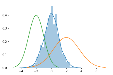
NOTE: As shown in diagram above there can be multiple mean μ, but we need to find the combination of mean μ and standard deviation σ which fit's the data.

As we know normal distribution has two parameters mean μ and standard deviation σ.

Now we need to find the value of mean μ and standard deviation σ such that the probability of X is maximized. Let's state it as P(X, μ, σ).  Or in general, let's define it in terms of ø P(X, ø).

J(ø) = P(X, ø) = P(X₁, X₂, X₃, . . . , X_n, ø)

Here we need to find the value of theta for which P(X, ø) is maximized. Let's define the MLE in a general way and then we look at how to specialize it in terms of Normal or Bernoulli Distribution. We will take two steps to make the calculation of cost function simpler:

1. The assumption that X₁ to X_n are independent:
It means that all the samples selected are at random and the selected sample doesn't have any relationship with other data points available. Since the samples are independent we can write J(ø) = P(X, ø) as a product. where L(ø) represents the likelihood with respect to theta:

$$ L(\theta) = {\prod_{i=1}^Np(x_i, \theta)}$$

2. Log to simplify the calculation:
The second step which we will take to simplify the calculation is that we will take a log on both sides.

$$ l(\theta) = L(\theta)= {\sum_{i=1}^Np(x_i, \theta)}$$

The above equations we have defined are the general equation of MLE. Now let's specialize them for continuous and discrete distribution.

Maximum Likelihood Estimation for a continuous distribution

Before defining the MLE for continuous distribution, let's define probability density function for normal distribution (since continuous variables follows normal distribution):

$$f(x) = {1 \over {\sigma \sqrt{2\pi}}}e^-{(x-\mu)^2 \over 2\sigma^2}$$

Now that we know the probability density function of the normal distribution, let's define the MLE for continuous distribution:

$$p(x_i, \theta) = {p(x_i,\mu, \sigma)}$$

$$ = {1 \over {\sigma \sqrt{2\pi}}}e^-{(x-\mu)^2 \over 2\sigma^2}$$

Taking log on both sides:

$$ \ln (p(x_i, \theta)) = \ln{1 \over {\sigma \sqrt{2\pi}}}-{(x_i-\mu)^2 \over 2\sigma^2}$$

$$ J(\mu, \sigma) = \sum_{i=1}^N\ln{1 \over {\sigma \sqrt{2\pi}}}-{(x_i-\mu)^2 \over 2\sigma^2}$$

$$ J(\mu, \sigma) = -\sum_{i=1}^N\ln ({\sigma \sqrt{2\pi})}-{(x_i-\mu)^2 \over 2\sigma^2}$$

Let's differentiate the cost function with respect to mean μ and standard deviation σ:

Differentiation with respect to mean μ:

$$\frac{\partial J}{\partial \mu}(0  -\sum_{i=1}^N{(x_i-\mu)^2 \over 2\sigma^2}) = 0$$

$$ {-1 \over 2\sigma^2} {\sum_{i=1}^N2{(x_i-\mu)(-1)}}= 0$$

$$  {\sum_{i=1}^N{x_i}}=  {\sum_{i=1}^N{\mu}} = N\hat\mu$$

$$ \hat\mu = \sum_{i=1}^N{x_i\over N} $$

Differentiation with respect to standard deviation σ, we will get:

$$  \hat\sigma = \sqrt{\sum_{i=1}^N{(x_i - \hat\mu)}^2\over N}$$

We use this is as an MLE function for the Linear Regression.

Maximum Likelihood Estimation for a discrete distribution

The Bernoulli distribution models events with two possible outcomes: success or failure. So Bernoulli distribution discrete in nature. So here we will find MLE for a discrete distribution by finding the parameters of a Bernoulli Distribution.

NOTE: Binary logistic regression problem is also a Bernoulli distribution.

The probability density function (pdf) for Bernoulli distribution is:

$$ p^x(1-p)^{1-x}$$

Now that we know the probability density of the Bernoulli distribution, let's define the MLE for discrete distribution. Here we will define the cost function in terms of p:

$${ ln(p) = ln(p^{y_i}(1-p)^{1-y_i})}$$

$$={\sum_{i=1}^N{y_i ln (p)} + (1-y_i) ln(1-p)}$$

Differentiation with respect to p, we will get:

$$\frac{\partial ln(p)}{\partial p} = 0$$

$$={\sum_{i=1}^N[{{y_i \over p} + {(1+y_i)(-1) \over (1-p)}}]}$$

This can be rewritten as,

$$={{1 \over p} \sum_{i=1}^N{{y_i}} - {1\over (1-p)}\sum_{i=1}^N(1-y_i) }$$

where, \(\sum_{i=1}^Ny_i\) represents the probability of success (P_S) and \(\sum_{i=1}^N (1 - y_i\)) represent the probability of failure (P_F)

Substituting value in the equation:

$$ {p \over (1-p)} = {P_S \over P_F}$$, which is also equal to \(p = {P_S \over N}\), which implies number of success over total number of observations. 

Maximum Likelihood Estimation for a logistic function

As said earlier, MLE for a logistic function is almost the same as MLE for discrete distribution. The only change moving to MLE for Logistic is that we calculate probability in the presence of other features.

Earlier we have seen in Bernoulli Distribution that,

$$ln(p) = {\sum_{i=1}^N{y_i ln (p)} + (1-y_i) ln(1-p)}$$

Now, for Logistic Regression we will change p = p(x_i) where x_i represents the independent variables:

$$={\sum_{i=1}^N{y_i ln (p/x_i)} + (1-y_i) ln((1-p/x_i))}$$

So the cost function of Logistic function can be rewritten as a function of ø:

$$J(\theta)={-1\over N}{\sum_{i=1}^N{y_i ln (h\theta(x(i)))} + (1-y_i) ln(1 - h\theta(x(i)))}$$

, where \(h\theta(x(i)) = {1 \over {1 + e^-{(\beta_0 + \beta_1x_i)}}}\)

Estimating the parameters via Iterative techniques

Amazing! We have defined the cost function for the logistic regression. The only pending thing to discuss is how obtain the best fit parameters such that cost function for logistic regression is maximized. To achieve this we have two different ways:

• Gradient Descent
• Newton's Method

Let's discuss them next.

Gradient Descent

Gradient descent method (first-order technique) is an iterative technique to solve for the betas. We have already defined the cost function of logistic regression as:

$$J(\theta)={-1\over N}{\sum_{i=1}^N{y_i ln (h\theta(x(i)))} + (1-y_i) ln(1 - h\theta(x(i)))}$$

NOTE: Cost function of logistic regression is designed to be like a bowl shape.

Now we have to find the global minimum of the function. In order to do this, we start off with one point and repeat unless we reach the minimum.

$$\theta_j : \theta_j - \alpha\ \frac{\partial J(\theta)}{\partial \theta_j}$$

And repeat the below step until we reach the minimum of the cost function.

$$\theta_j : \theta_j - \alpha {\sum_{i=1}^N(h\theta(x^i) - y_i)x_j^i}$$

Newton-Raphson Method

Newton-Raphson Method (second-order technique) is an alternative to Gradient Descent and we reach the same result as with Gradient Descent. Newton-Raphson Method is the same as that of Gradient Descent.

Consider again the cost function for logistic regression:

$$J(\theta)={-1\over N}{\sum_{i=1}^N{y_i ln (h\theta(x(i)))} + (1-y_i) ln(1 - h\theta(x(i)))}$$

and the goal is to find \(\theta\) for which \(J(\theta)\) is minimized. (i.e. Cost function is minimized). To do this we take derivative of cost function and equate it to 0.

$$ \frac{\partial J(\theta)}{\partial \theta} = 0$$

Intutively, what Newton-Raphson method do is:

• It calculate the first derivative of the cost function and starts with some random value of theta.
• Then the tangent is drawn for the theta value and extended till the x-axis.
• Next time the theta value is chosen where the tangent has intersected the x-axis.
• The same process is repeated unless and until the first derivative of the cost function is zero.

Because of this Newton-Raphson Method converges very quickly as compared to the gradient descent method. Now having an intuitive understanding of the algorithm let's see mathematical how to move from one theta value to another.

Let say the distance between \(\theta_0\) and \(\theta_1\) is \(\delta\). Therefore \(\delta\) is represented as:

$$ \delta = {J^{'}(\theta) \over J^{''}(\theta)}$$

using pythagoras theorem, where first differential of cost function is height, second differential of cost function is hypotenuse and  \(\delta\) is the width.

Hence we conclude that,

$$ \theta^{t+1} = \theta^t - {J^{'}(\theta^{(t)}) \over J^{''}(\theta^{(t)})}$$

The above equation represent Newton-Raphson Method. There is more genralized way of representing the same:

$$\theta_t : \theta_t - H^{-1}\ \frac{\partial J(\theta)}{\partial \theta_t}$$

where \(H^{-1}\) represent the Hessian matrix. And \(H_{ij}\) is represented as,

$$H_{ij} = \frac{\partial^2 J}{\partial \theta_i \partial \theta_j}$$

Python Implementation

Congratulations! You have understood the important concept required to solve problems using logistic regression. Now let's look at the python implementation of it using packages.

First, let's start with the stats model package and find β0 and β1 using it

import statsmodels.api as sm
from sklearn.datasets import load_iris

X, y = load_iris(return_X_y=True)

logm1 = sm.GLM(y,(sm.add_constant(X)), family = sm.families.Binomial())
logm1.fit().summary()

We can also use the sklearn package to achieve the same task. Let's look at the code shown below:

from sklearn.datasets import load_iris
from sklearn.linear_model import LogisticRegression

X, y = load_iris(return_X_y=True)

clf = LogisticRegression(random_state=0, solver='lbfgs', multi_class='multinomial').fit(X, y)
clf.predict(X[:2, :])

Here, in the example shown above, we have trained the sklearn Logistic Regression model with few hyperparameters.

Linear Equation of Sigmoid function

The equation of logistic regression is denoted as:

$$ P = {1\over {1 + e^{-(\beta_0 + \beta_1x)}}}$$

The logistic regression equation is correct but it is not very intuitive. (i.e It is very difficult to have a visual understanding of the relationship between P and x)

So we need to convert equation to a slightly different format for better understanding. We start with subtracting 1 from both the sides.

$$ 1 - P = {e^{-(\beta_0 + \beta_1x)}\over {1 + e^{-(\beta_0 + \beta_1x)}}}$$

Let's divide the first and second equation:

$$ {P \over 1 - P} = e^{(\beta_0 + \beta_1x)}$$

Let's take log on both sides:

$$ ln({P \over 1 - P}) = (\beta_0 + \beta_1x)$$

where, \(P \over 1 - P\) is odds and \(ln ({P \over 1 - P})\)  is log odds.

So, now, instead of probability, you have odds and log odds. Clearly, the relationship between them and x is much more intuitive and easy to understand. The relationship between x and log odds is linear.

If we plot log odds and x for the fixed value of \(\beta_0\) and \(\beta_1\) the relationship will be linear. 

Therefore, many times it makes sense to present a logistic regression model’s results in terms of log-odds or odds than to talk in terms of probability.

Other Forms of logistic regression

So far we have seen the logit form of logistic regression, which is denoted as:

$$P =  {1\over {1 + e^{-(\beta_0 + \beta_1x)}}}$$

links = sm.families.linkslogm = sm.GLM(y_train,(sm.add_constant(X_train)),
family= sm.families.Binomial(link=links.logit))logm.fit().summary()

However, there are other forms of logistic regression as well:

• probit form of logistic regression
• cloglog form of logistic regression

Let's discuss them next.

probit form of logistic regression

The probit form of logistic regression is represented as:

$$P = \phi^{-1}(\beta_0 + \beta_1 x)$$

And the python code to use probit form is as shown below:

links = sm.families.linkslogm = sm.GLM(y_train,(sm.add_constant(X_train)),
family=sm.families.Binomial(link=links.probit))logm.fit().summary()

cloglog form of logistic regression

The cloglog form of logistic regression is represented as:

$$P = ln(-ln(1 - (\beta_0 + \beta_1 x)))$$

And the python code to use cloglog form is as shown below:

links = sm.families.linkslogm = sm.GLM(y_train,(sm.add_constant(X_train)),
family=sm.families.Binomial(link=links.cloglog))logm.fit().summary()

More in the form of logistic regression will be covered in later posts.

Multivariate Logistic Regression

There is not much change when moving from univariate to multivariate logistic regression. In multivariate there will be more than one independent variable which will help to predict the target variable. The sigmoid curve of multivariate logistic regression is represented as:

$$ P = {1\over {1 + e^{-(\beta_0 + \beta_1x_1 + \beta_2x_2 + . . . . . . . + \beta_nx_n  )}}}$$

I want to leave you here with an open question: As we have seen that we can perform logistic regression on data having like Bernoulli Distribution which means the target variable can have only two outcomes: failure and success. Is it possible to apply logistic regression on a dataset having more than 2 classes in target variables? Share your views in the comment section below.

Summary

In this post, we have started understanding why we need Logistic Regression for classification problems. We defined the cost function for the Logistic regression algorithm and saw the python implementation using stats model and sklearn packages.

We discussed the linear equation of the logistic regression which is much more intuitive to understand. We also discussed various forms of logistic regression. And saw what got changed when moving from simple logistic regression to multivariate logistic regression.