Distributional Semantics: Techniques to represent words as vectors

April 18, 2025

The distributional hypothesis states that the context words of the given ambiguous word determine the correct meaning of the word. Which in simple terms means that the meaning of the given word can be determined in the context (or neighboring words) in which the word is used.
There are multiple techniques available to understand the meaning of the word based on context. In this post, we will be covering one of the most popular techniques which is word embeddings but before going there we will first understand the occurrence matrix and co-occurrence matrix which will help us realize the beauty behind the word embedding technique.
Let's get started and understand various techniques to represent the words as vectors to understand the meaning of the word in the context a word is used.
Occurrence Matrix
An occurrence matrix also called a term-occurrence context matrix is a technique where each row is a term and each column represents an occurrence context. And, the context depending on the application we are designing can be a sentence, paragraph, tweet, comment, etc.
The diagram shown below represents the occurrence matrix where the row is defined as a term distributional vector and the column is defined as a context or document distributional vector.

There are different methods using which we can capture the weight of the occurrence of a term in a given document or context i.e., \(F_{n,n}\) as represented in the diagram above. Different ways include:
- Distributional Incidence Matrix: This is the simplest way where we record if the term has occurred in the context or not. The matrix \(F_{i,j}\) return 1 if \(t_{i}\) occurs in \(c_{j}\), else the value is 0.
- Distributional Frequency Matrix: This is a sort of normalized form where we calculate the frequency of terms occurring in the context and divide by the term occurring in any context. The matrix \(F_{i,j}\) is defined as \(tf_{i,j}\) which is equal to \(0.5 + 0.5{freq_{t_i, c_j} \over max_t freq_{t, c_j}}\).
- Distributional Relevancy Matrix: This is based on the tf-idf which represents the term frequency and inverse document frequency. The matrix \(F_{i,j}\) is defined as \(tf_{i,j}.idf_i\) where \(idf_i\) is defined as \(log{|C|\over |C_{t_i}|}\) where \(|C|\) is the number of occurrence context and \(|C_{t_i}|\) is the number of contexts where \({t_i}\) has occurred.
The distributional frequency and distributional relevancy matrix might be a better representation than the vanilla incidence matrix as it will give lower weights to more frequent words. For example, in a word-sentence matrix, if many sentences contain the word ‘might’ (which is not a stopword since it is also a noun), the word ‘might’ will be assigned a lower weight, after discounting for its frequent occurrence.
Example
Let us understand the occurrence matrix with the help of an example. Consider four documents each of which is a paragraph taken from a movie. Assume that the vocabulary has only the following words: fear, beer, fun, magic, and wizard.
The table below summarises the term-document matrix, each entry representing the frequency of a term used in a movie:
| Harry Potter and the Sorcerer's Stone | The Prestige | Wolf of Wall Street | Hangover | |
| fear | 10 | 8 | 2 | 0 |
| beer | 0 | 0 | 2 | 8 |
| fun | 6 | 5 | 8 | 8 |
| magic | 18 | 25 | 0 | 0 |
| wizard | 20 | 8 | 0 | 0 |
NOTE: The dot product of two vectors is large if the two vectors are ‘similar’ to each other.
The vector for "Harry Potter and the Sorcerer's Stone" is (10,0,6,18,20) and the vector for "The Prestige" is (8,0,5,25,8). The dot product will be (10,0,6,18,20)*(8,0,5,25,8) = 80 + 30 + 450 + 160 = 110 + 450 + 160 = 720. In the same way, we can calculate the dot product of other movies and will find that the dot product is smaller. Therefore, we can conclude that the movies "Harry Potter and the Sorcerer's Stone" and "The Prestige" are similar.
Similarly, we can find the dot products for terms as well. For example, the vector for "magic" is (18,25,0,0) and the vector for the "wizard" is (20,8,0,0). The dot product will be (18,25,0,0)*(20,8,0,0) = 360 + 200 = 560. In the same way, we can calculate the dot product of other words and will find that the dot product is greater than the dot product of any other terms. Therefore we say that these two terms are the most similar to each other.
Use cases
Term-document matrix (or occurrence context matrix) are commonly used in tasks such as information retrieval. Two documents having similar words will have similar vectors, where the similarity between vectors can be computed using a standard measure such as the dot product. Thus, we can use such representations in tasks where, for example, we want to extract documents similar to a given document from a large corpus.
Limitations
A real term-document matrix will be much larger and sparse, i.e. it will have as many rows as the size of the vocabulary (typically in tens of thousands) and most cells will have the value 0 (since most words do not occur in most documents). Therefore will be challenging to perform operations.
Further, using the term-document matrix to compare similarities between terms and documents poses some serious shortcomings such as with polysemic words, i.e. words having multiple meanings. For example, the term ‘Java’ is polysemic (coffee, island, and programming language), and it will occur in documents on programming, Indonesia, and cuisine/beverages.
So if we imagine a high dimensional space where each document represents one dimension, the (resultant) vector of the term ‘Java’ will be a vector sum of the term’s occurrence in the dimensions corresponding to all the documents in which 'Java' occurs. Thus, the vector of ‘Java’ will represent some sort of an ‘average meaning’, rather than three distinct meanings (although if the term has a predominant sense, e.g. it occurs much more frequently as a programming language than its other senses, this effect is reduced).
Next, let us understand an alternate way to generate a distributed representation of words using the term-term co-occurrence matrix.
Co-occurrence Matrix
The co-occurrence matrix also called term-term co-occurrence matrix is a technique that is a square matrix having terms in both rows and columns. This is a symmetric square matrix. Unlike the occurrence matrix, where each column represents a context (such as a document), now in the co-occurrence matrix the columns also represent a word.
There are different ways of creating a co-occurrence matrix. Let's see the most popularly used ones:
- Using the occurrence context: We divide the corpus into occurrence contexts. If two terms occur in the same context, they are said to have occurred in the same occurrence context.
For example, If we take a sentence as an occurrence context and after doing preprocessing (removal of stop words, lemmatization., etc.) all the terms occurring in the same sentence will be marked as they co-occur with each other. And, words in different sentences will have different contexts.
- Skip-grams (x-skip-n-grams): A sliding window will include the (x+n) words. This window will serve as the context now. Terms that co-occur within this context are said to have co-occurred.
For example, the 3-skip-2-gram model means that we can select 2 words, and we can skip three or fewer words in between the selected two words.
Similar to the occurrence matrix, in the co-occurrence matrix as well we also get the term distributional vector across the terms which is an abstract representation of the neighbour of the words.
In a term-document matrix or occurrence matrix, we have used the dot product of two vectors to compare the similarities between vectors. For the co-occurrence matrix, we have two different metrics that we can use to compare the similarity between two different metrics.
- \(L_p\) Norm: Given two-term vectors \({t_i} = (f_{i, 1}, f_{i, 2}, . . . , f_{i, n})\) and \({t_j} = (f_{j, 1}, f_{j, 2}, . . . , f_{j, n})\) we compare the distance between them to compare the neighborhood of the terms. The small distance\(L_p(t_i, t_j) = \sqrt[p]\sum_{k=1}^n (|f_{j,k} - f_{i,k}|)^p\) represents the similarity between two-word vectors. Not only measure the similarity but also measure the magnitude of words being used.
We have a family of norms using which we can compare the distance as given below:- Manhattan Distance (\(L_1\) norm) where p is 2.
- Euclidean Distance (\(L_2\) norm) where p is 2.
- Cosine Similarity: This technique calculates the angle \(cos(t_i, t_j) = {t_i . t_j \over ||t_i|| ||t_j||} = {\sum_{k=1}^n f_{i,k} . f_{j,k}\over {\sqrt(\sum_{k=1}^nf_{i,k}^2)\sqrt(\sum_{k=1}^nf_{j,k}^2)}}\) between the two term vectors. The cosine similarity ranges between 0 to 1. The angle between two similar words will be very small and the cosine of the angle will be high for similar words.
Limitations
One shortcoming of the simple co-occurrence-based approach (where a context is defined as a sentence) is that words appearing in different sentences though close to each other will not reflect in the term-term matrix. Also, the matrix will be sparse and the dimensionality of each vector will be quite high (as big as the vocabulary of the corpus).
Example
Consider we have vocabulary such as "Man stumbled seconds Dursley cloak upset knocked ground". We want to create a co-occurrence matrix using this paragraph using the 3-skip-2-gram technique. The co-occurrence pairs that we get would be:
- (Man, stumbled) (stumbled, seconds) (seconds, Dursley) (Dursley, cloak) (cloak, upset) (upset, knocked) (knocked, ground)
- (Man, seconds) (stumbled, Dursley) (seconds, cloak) (Dursley, upset) (cloak, knocked) (upset, ground)
- (Man, Dursley) (stumbled, cloak) (seconds, upset) (Dursley, knocked) (cloak, ground)
- (Man, cloak) (stumbled, upset) (seconds, knocked) (Dursley, ground)
Now we fill the co-occurrence matrix with 1 if a word pair exists in the above co-occurrence pairs and we get a co-occurrence matrix.
| Man | stumbled | seconds | Dursley | cloak | upset | knocked | ground | |
| Man | 1 | 1 | 1 | 1 | 1 | 1 | 1 | 1 |
| stumbled | 1 | 1 | 1 | 1 | 1 | 0 | 0 | 0 |
| seconds | 1 | 1 | 1 | 1 | 1 | 1 | 0 | 0 |
| Dursley | 1 | 1 | 1 | 1 | 1 | 1 | 1 | 0 |
| cloak | 1 | 1 | 1 | 1 | 1 | 1 | 1 | 1 |
| upset | 1 | 0 | 1 | 1 | 1 | 1 | 1 | 1 |
| knocked | 1 | 0 | 0 | 1 | 1 | 1 | 1 | 1 |
| ground | 1 | 0 | 0 | 0 | 1 | 1 | 1 | 1 |
- What is the L2 distance between the words 'man' and 'Dursley'? The vector for man is (1,1,1,1,1,1,1,1) and the vector for Dursley is (1,1,1,1,1,1,1,0). (Square of L2 norm) is the sum of the square of individual terms of (vector for a man - vector for Dursley) = (0 + 0 + 0 + 0 + 0 + 0 + 0 + 1) = 1
- 'Knocked' and 'ground' are similar words as the distance between them is smaller as compared to other words. Vector for knocked = (1,0,0,1,1,1,1,1), vector for ground = (1,0,0,0,1,1,1,1). Cosine Similarity between these two vectors = (1+0+0+0+1+1+1+1)/squareroot(6*5)=5/squareroot(30).
The occurrence and co-occurrence matrix have really large dimensions (equal to the size of the vocabulary V). This is a problem because working with such a huge matrix makes them almost impractical to use. Let's understand how to tackle this problem next with word embeddings.
Word Embeddings
Since the occurrence and co-occurrence matrix is sparse and high-dimensional probable question comes to mind, why not reduce the dimensionality using matrix factorization techniques such as SVD, etc.?
This is exactly what word embeddings aim to do. Word embeddings are a compressed, low-dimensional version of the mammoth-sized occurrence and co-occurrence matrix. Word embedding reduces the noise in the word vectors generated using occurrence and co-occurrence matrix techniques.
Each row (i.e. word) has a much shorter vector (of size say 100, rather than tens of thousands) and is dense, i.e. most entries are non-zero (and we still get to retain most of the information that a full-size sparse matrix would hold). A few popular algorithms for word embeddings include Word2vec or GloVe.
Different approaches to further refine the occurrence and co-occurrence matrix to generate word embeddings (i.e. reducing the dimension of the word vectors) are:
- Frequency-based approach: Reducing the term-document matrix using a dimensionality reduction technique such as SVD. Example: LSA.
- Prediction-based approach: In this approach, the input is a single word (or a combination of words) and the output is a combination of context words (or a single word). A shallow neural network learns the embeddings such that the output words can be predicted using the input words. Example: Skip-gram, CBOW (Continuous Bag of Words).
Let's understand both of the above-mentioned approaches technique in detail, and start with the frequency-based approach i.e., LSA.
Latent Semantic Analysis (LSA)
It is a frequency-based approach to generating word embeddings. It uses Singular Value Decomposition (SVD) to reduce the dimensionality of the matrix. Any term context matrix can be re-written as
$$A_\text{m x n} = U_\text{m x r} . \Sigma_\text{r x r}. V_\text{n x r}^T $$
where r is the rank of the matrix which means the number of rows in the matrix that are linearly independent of each other. The rank or columns in the decomposed matrix represent the combination of the original terms (i.e. as a linear combination of columns of matrix A). Refer to the post, Principal Component Analysis Detailed Explanation to understand the working of PCA in detail.
In LSA, we take a noisy higher dimensional vector of a word and project it onto a lower dimensional space. The lower dimensional space is a much richer representation of the semantics of the word.
Singular vectors in LSA are the ones where the points on the vector space do not change their position after projecting onto lower dimensional space.
LSA Use cases
- LSA is widely used in processing large sets of documents for various purposes such as document clustering and classification (in the lower dimensional space).
- Comparing the similarity between documents (e.g. recommending similar books to what a user has liked).
- Finding relations between terms (such as synonymy and polysemy), etc.
Limitations of LSA
- The resulting dimensions are not interpretable (the typical disadvantage of any matrix factorization-based technique such as PCA).
- LSA cannot deal with issues such as polysemy. For example, consider the term ‘Python’ has three senses (Programming Language, Snake, and Island), and the representation of the term in the lower dimensional space will represent some sort of an ‘average meaning’ of the term rather than three different meanings.
Let's look at Python code to implement LSA using TfidfVectorizer and TruncatedSVD.
import nltk
from sklearn.feature_extraction.text import TfidfVectorizer
from sklearn.decomposition import TruncatedSVD

TextCorpus = ['Seven continent planet',
'Five ocean planet',
'Asia largest continent',
'Pacific Ocean largest',
'Ocean saline water']

text_tokens = [sent.split() for sent in TextCorpus]

transformer = TfidfVectorizer()
tfidf = transformer.fit_transform(TextCorpus)

svd = TruncatedSVD(n_components = 3)
lsa = svd.fit_transform(tfidf)
print(lsa)

# Output
array([[ 5.69995606e-01, -5.21026572e-01,  4.81700519e-01],
       [ 6.29788097e-01,  2.47716942e-01,  5.41216825e-01],
       [ 5.69995606e-01, -5.21026572e-01, -4.81700519e-01],
       [ 6.29788097e-01,  2.47716942e-01, -5.41216825e-01],
       [ 4.08516626e-01,  6.90173499e-01,  2.14324675e-15]])
In the code demonstrated above, we started with a sample corpus and represented the corpus in tf-idf format. Thereafter, TruncatedSVD is used which is an implementation of LSA where the number of documents was kept constant and the column size was reduced to 3, where columns represented the terms. The 'lsa' object defined in the code will now have a semantic representation of each document in reduced dimensional space.
In the code shown above, the number of documents was kept constant and the column size was reduced, where columns represented the terms. Next, let's observe how we can generate a vector of the words using LSA by keeping the number of terms constant while reducing the number of rows (i.e. documents).
from sklearn.decomposition import TruncatedSVD

svd = TruncatedSVD(n_components = 3)

# using the same tfidf object defined in previous code
lsa = svd.fit_transform(tfidf.T)
print(lsa)

# Output
array([[ 2.96093980e-01,  3.21358058e-01,  3.09860265e-01],
       [ 4.77773518e-01,  5.18539316e-01,  4.45858570e-15],
       [ 3.42561592e-01, -1.59982023e-01, -3.64540860e-01],
       [ 5.15263294e-01,  1.30197169e-01,  5.44102582e-01],
       [ 5.96632444e-01, -4.90698274e-01, -3.78297676e-15],
       [ 3.42561592e-01, -1.59982023e-01,  3.64540860e-01],
       [ 5.15263294e-01,  1.30197169e-01, -5.44102582e-01],
       [ 2.05756406e-01, -4.12736768e-01, -3.84291116e-15],
       [ 2.96093980e-01,  3.21358058e-01, -3.09860265e-01],
       [ 2.05756406e-01, -4.12736768e-01, -3.84291116e-15]])
In the above code, we are using the same tf-idf that we have generated in the previous code. But this time, we are generating the vectors of each word rather than generating vectors for each document.
Next, let us explore prediction-based techniques to generate word embeddings.
Skip-gram Model
It is a prediction-based approach that uses the current word to predict the words in the neighborhood and help generate word embeddings. In this approach to generating word vectors, the input is the target word and the task of the neural network is to predict the context words (the output) for that target word i.e., It uses the current word to predict the words in the neighborhood. For example, consider the sentence, "what will be will be".
The skip-gram training set for the given sentence will be:
([will], what), ([what, be], will), ([will, will], be), ([be, be], will), ([will], be)
The training set is created considering a word e.g., 'will', and checking the words that surround the given word. e.g., 'what' and 'be' as represented in the image below.
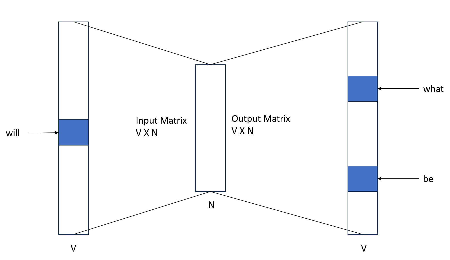
For skipgram, the size of the input and the size of the output that we get is of size of vocabulary V. In the input vector, we will have all zeros except the input word that we are passing and the same applies to the output layer as well.
Next, the obvious question is, how skip-gram works?
The skip-gram model has one hidden layer that connects the input and output layers. The input layer is connected to the hidden layer where all neurons are given random weights and the task is to learn these weights to give accurate output i.e., the words surrounding the given word.
Further, the input word is represented in the form of a 1-hot-encoded vector. Once trained, the weight matrix between the input layer and the hidden layer gives the word embeddings for any target word (which is part of the vocabulary on which the skip-gram algorithm is trained).
The neural network used for skip-gram is informally called 'shallow' because it has only one hidden layer, though one can increase the number of such layers. Such a shallow network architecture was developed by Google to train word embeddings for about 1.6 billion words, which became popularly known as Word2Vec.
Example
Let us consider an example where we have a large corpus of vocabulary |V| = 10,000 words to understand how the skip-gram model works. The task is to create a word embedding of 300 dimensions for each word (i.e. each word should be a vector of size 300 in this 300-dimensional space).
The first step is to create a distributed representation of the corpus using a technique such as skip-gram where each word is used to predict the neighboring 'context words'. The task of the neural network is to learn to predict the context words correctly for each input word. The input to the network is a one-hot encoded vector representing one term. For example, the figure below shows an input vector for the word ‘ants’.
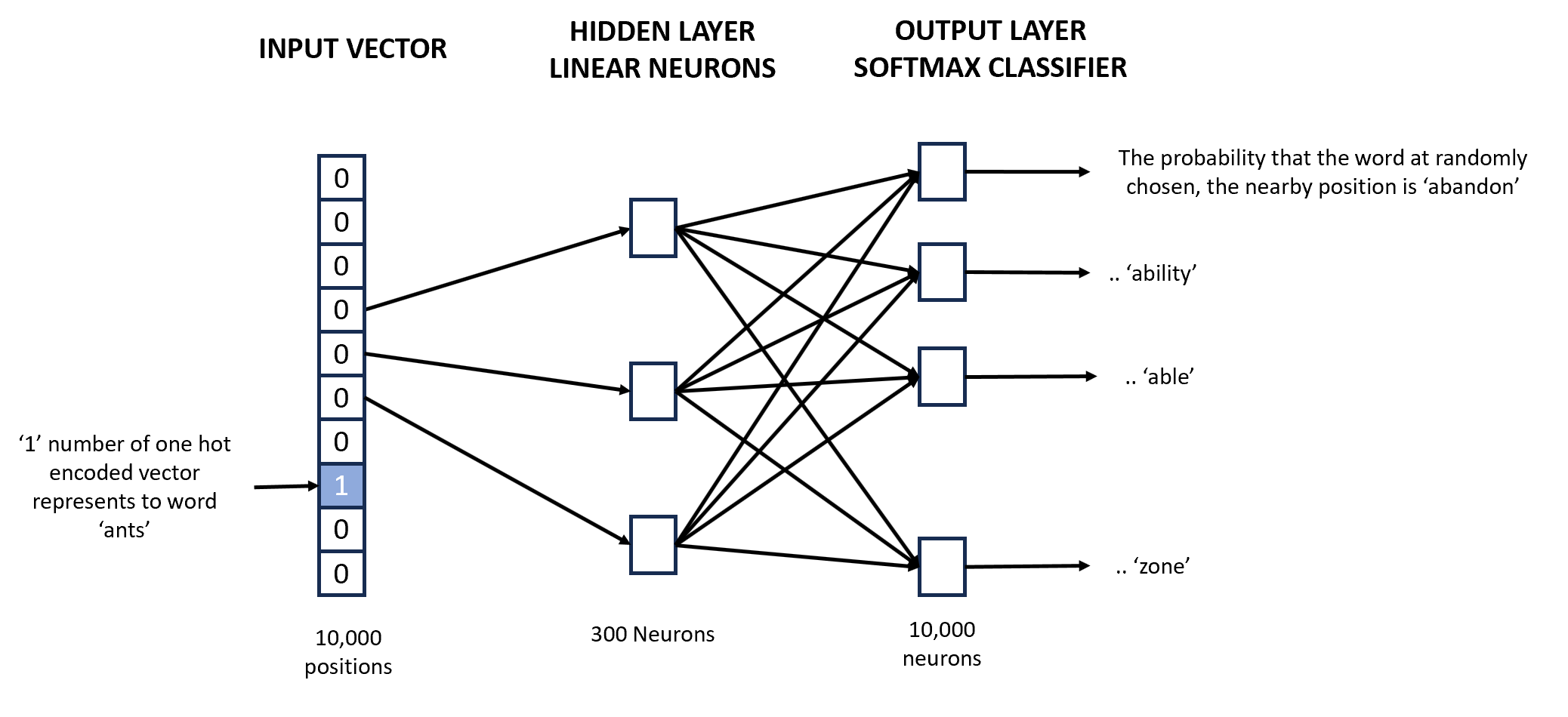
If the context words for the word ‘ants’ are ‘bite’ and ‘walk’, the elements corresponding to these two words should have much higher probabilities (close to 1) than the other words. The hidden layer is a layer of 300 neurons. Each of the 10,000 elements in the input vector is connected to each of the 300 neurons (though only three connections are shown above). Each of these 10,000 x 300 connections has a weight associated with it. This matrix of weights is of size 10,000 x 300, where each row represents a word vector of size 300.
The cost function of the network is thus the difference between the ideal output (probabilities of ‘bite’ and ‘walk’) and the actual output (whatever the output is with the current set of weights). Once such a network is trained, each of the 10,000 words will have a word embedding of size 300.
Let us explore Python implementation to generate word embedding using the Word2Vec algorithm.
import nltk
from gensim.models.word2vec import Word2Vec

TextCorpus  = ["My name is Tavish Aggarwal",
               "Tavish loves to code and solve business problems",
               "Tavish is certified Data Scientist",
               "Delhi is capital of India",
               "I like ML"
]

text_tokens = [sent.split() for sent in TextCorpus]

model = Word2Vec(text_tokens,min_count=1, vector_size = 100, sg=1)

# To generate word embeddings of words that are in the vocabulary
model.wv['Tavish']

# To find a similar word to a given word using the Cosine similarity
model.wv.most_similar("Tavish",topn=5)
When generating word embeddings using the Word2Vec gensim algorithm, the default vector size for word embeddings is 100, but one can reduce or increase the vector size, though reducing the vector size will have an impact on the goodness of word vectors. We are also passing the 'sg' parameter as 1, which means we are learning with one neighbor (i.e., skip-gram).
Continuous-Bag-of-Words (CBOW) model
Apart from the skip-gram model, there is one more prediction-based approach model that can be used to extract word embeddings for the word. This model is called the Continuous-Bag-of-Words (CBOW) model and generates embeddings faster than the skip-gram model.
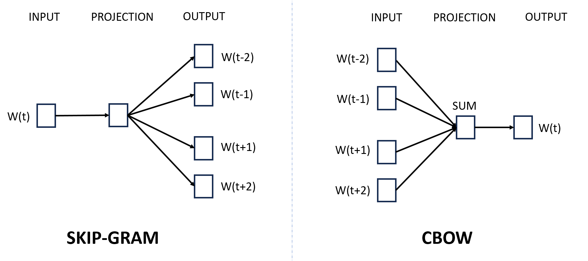
Recall that skip-gram takes the given word as the input and predicts the context words (in the window), whereas CBOW takes the context terms as the input and predicts the target/given term. This is how the CBOW algorithm is different from the skip-gram model.
model = Word2Vec(text_tokens,min_count=1, vector_size = 100, sg=0, window=5)By default, the sg parameter is 0 which means it is using the CBOW approach to calculate word embeddings. To use the skipgram approach we need to specify the sg value greater than 0.
One more difference between skip-gram and CBOW is that, in CBOW the vectors from the context words are averaged before predicting the center word. In skip-gram, there is no averaging of embedding vectors. Because of this, the skip-gram model can learn better representations for the rare words when their vectors are not averaged with the other context words in making the predictions. This means, that even though skip-gram is slow in performance but much more accurate as compared to CBOW.
In CBOW we also use the 'window' parameter which specifies the context window (we don't use the window in skip-gram). The context window of 5 as shown in the example above simply means, that five word to the left of the given word and five words to the right of the given word is considered to generate word embeddings. Therefore, when we choose a small window size (such as 5), similar words will often be synonyms (For example queen and monarch as they are similar), whereas if we choose a larger window size (such as 10), similar words will be contextually similar words (For example, king, queen, and throne will be similar as they appear in similar context).
GloVe and FastText Model
A few other word embedding techniques were developed such as GloVe (Global Vectors for Words) developed by a Stanford research group, or fastText developed by Facebook AI Research (FAIR), etc.
from gensim.scripts.glove2word2vec import glove2word2vec
from gensim.models.keyedvectors import KeyedVectors

glove_input_file = 'glove.6B.100d.txt'
word2vec_output_file = 'glove.6B.100d.w2vformat.txt'
glove2word2vec(glove_input_file, word2vec_output_file)

glove_model = KeyedVectors.load_word2vec_format("glove.6B.100d.w2vformat.txt", binary=False)

glove_model.most_similar("king")
In the Python code shown above, we use pre-trained word embeddings, which are trained on about 6 billion unique tokens and are available as pre-trained word vectors ready for text applications. These embeddings can be obtained from the GloVe website.
Effect of Context
The training corpus also has a significant effect on what the embeddings learn. For example, if we train word embeddings on a dataset related to movies and financial documents, they would learn very different terms and semantic associations. While working with word embeddings one has two possible options:
Training your word embeddings: This is suitable when one has a sufficiently large dataset (a million words at least) or when the task is from a unique domain (e.g. healthcare). In specific domains, pre-trained word embeddings may not be useful since they might not contain embeddings for certain specific words (such as drug names).
Using pre-trained embeddings: Generally speaking, we should always start with pre-trained embeddings. They are an important performance benchmark trained on billions of words. We can also use the pre-trained embeddings as the starting point and then use the text data to further train them using the transfer learning approach.
BONUS: Using word embeddings for the classification task
The Jupyter Notebook demonstrates how to use the word embeddings for the classification task for the news article where the task is to classify the news articles into one of the eight different categories.
The notebook first demonstrates the basic bag-of-word technique and trains various algorithms such as Bernoulli Naive Bayes or Multinomial Naive Bayes for the classification task. The notebook also demonstrates word embedding techniques (using pre-trained embeddings such as GloVe and training embeddings on our own) that we have gone through in this post and then a logistic regression algorithm is trained on the generated word embeddings.
The notebook also demonstrated classification tasks and showed how word embedding can be used, though the same embeddings can be used for a wide variety of ML tasks. For example, say we want to cluster a large number of documents (document clustering), one can create a 'document vector' for each document and cluster them using (say) k-means clustering the word embeddings come in handy to achieve such tasks.
We can even use word embeddings in more sophisticated applications such as conversational systems (chatbots), fact-based question answering, etc. Word embeddings can also be used in other creative ways. The Jupyter Notebook demonstrates how word vectors can be modified to contain a 'sentiment score', which is then used to model tweet opinions.
Summary
In this post, we have covered two categories broad categories of techniques that can help understand the meaning of the text in the given context.
The term-document occurrence matrix is a technique where each row is a term in the vocabulary and each column is a document (such as a webpage, tweet, book, etc.). LSA is an example of an occurrence matrix. Whereas, the term-term co-occurrence matrix, where the \(i^{th}\) row and \(j^{th}\) column represent the occurrence of the \(i^{th}\) word in the context of the \(j^{th}\) word. It always has an equal number of rows and columns, because both rows and columns represent the terms in the vocabulary. HAL, Word2Vec, and GloVe are examples of co-occurrence matrix.
Thereafter we learned two different types of techniques to generate word embeddings. This includes frequency-based approaches such as LSA and prediction-based approaches such as skip-gram and CBOW (Continuous Bag of Words) algorithm.
Author Info