Decoding the Magic of Probabilistic Graphical Models: A Comprehensive Guide to Understanding and Applying PGMs in Data Science

Probabilistic Graphical models belong to the generative class of models which can model all the relationships between the variables and answer any question asked even when partial data is provided. They provide a flexible and intuitive framework for representing probabilistic relationships between variables present in the dataset.

PGMs come in two main flavors: Bayesian Networks and Markov Networks. Bayesian Networks are directed acyclic graphs that represent the probabilistic dependencies between variables. Markov Networks, on the other hand, are undirected graphs that represent the conditional independence relationships between variables.

This will be a lengthy post and can get overwhelming, therefore I suggest bookmarking this one and reading it in your free time. Let's get started and understand PGMs in depth.

Prerequisites

Probabilistic Graphical Models (PGMs) are a powerful tool for modeling complex systems and reasoning under uncertainty. We will be covering a few prerequisites before we deep dive into the understanding of probabilistic graphical models.

Joint Probability and Conditional Probability

A joint probability is the probability of two events taking place simultaneously. Simply put, it is the probability that event X occurs at the same time as event Y. 

The joint probability of two events X and Y is P(X በ Y) also represented as P(X, Y).
Formula:  P(X, Y) = P(X) * P(Y), if both events X and Y are independent of each other

Joint probability should not be confused with conditional probability, which is the probability that one event will happen given that another action or event happens.

The conditional probability of two events X and Y is represented as P(X | Y).
Formula: P(X|Y) = P(X በ Y) / P(Y) = P(X, Y) / P(Y)

Law of Total Probability

Before we move on to the Law of Total Probability, let's first understand what the multiplication rule is. The multiplication rule of probability states that the probability of occurrence of both events A and B is equal to

P(X ∩ Y) = P(X/Y). P(Y), if X and Y are dependent events. It is a corollary of the definition of conditional probability.

P(X ∩ Y) = P(X). P(Y), if X and Y are independent events

The Law of Total Probability is a fundamental rule in statistics relating to conditional and marginal probabilities. The rule states that if the probability of an event is unknown, it can be calculated using the known probabilities of several distinct events.

Consider an example where three events A, B, and C have occurred where events B and C are distinct from each other, while event A intersects with both events. Refer to the diagram shown below.

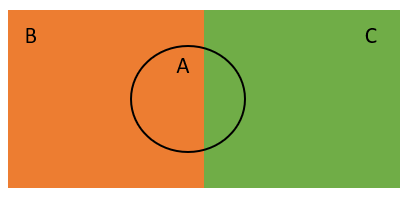
We do not know the probability of event A. However, we know the probability of event A under condition B and the probability of event A under condition C.

The total probability rule states that by using the two conditional probabilities, we can find the probability of event A as

$$P(A) = \sum_n P(A  \cap B_n)$$

The above equation is known as the total law of probability. Now using the multiplication rule we can substitute each term on the right-hand side of the equation and write it as follows:

$$P(A) = \sum_n P(A  | B_n) *P(B_n)$$

Bayes' Theorem

Bayes’ theorem describes the probability of an event, based on prior knowledge of conditions that might be related to the event. If we know the conditional probability P(B|A), we can use Bayes’ rule to find out the reverse probability P(A|B). Refer to the post, Naïve Bayes Algorithm Detailed Explanation to understand in detail. 

Graphs

A graph is a mathematical object consisting of a set of vertices or nodes, connected by a set of edges.

Graph theory concepts such as nodes, edges, paths, cycles, connectivity, and graph algorithms are all important for understanding the representation, inference, and learning algorithms used in PGMs. In PGMs, graphs are used as a visual representation of the probabilistic relationships between variables, and this post assumes that the reader has an understanding of graph theory as it is essential for working with these models.

Having an understanding of the prerequisites needed to understand the PGMs, let's move forward and dive into the main agenda of this post, PGMs.

Probabilistic Graphical Models

In this post, we will learn one of the generative classes of models which is Probabilistic Graphical Models. These classes of models have a variety of applications such as Medical or fault diagnosis; Computer vision: such as image segmentation, and 3D reconstruction; NLP: such as name-entity recognition, and topic modeling; and Time series problems: such as stock market predictions amongst many others. 

A Probabilistic Graphical Model, often referred to as PGM, is a generative algorithm that is an interplay of probabilistic and graphical models. Let us understand two terms probabilities and generative separately first.

What is the difference between the probabilistic and deterministic models?

In simple terms, any model that outputs probabilities is referred to as a probabilistic model. A key difference between a probabilistic and a non-probabilistic model is that in probabilistic models, the final decision is taken by the user of the model which is not the case with non-probabilistic models.

A few more examples of probabilistic models include Neural Networks with a softmax layer as the output layer or Logistic Regression.

A non-probabilistic or deterministic model like SVM would give the decision of the particular class to which the data point would belong while a probabilistic model like logistic regression would give the probability of the data point belonging to the different classes.

NOTE: It is important to note here that the confidence of the model in predicting the class of the data point is very different from the correctness of the model. The model may give a prediction with high probability, but can still be wrong i.e., not correct in the prediction.

What is the difference between the generative and determinative models?

So far we have understood what probabilistic models are and how they are different than deterministic models. Now, even among probabilistic models, there are two further classes of models which are generative and discriminative:

Discriminative models are trained to answer a specific question, such as predicting the label given some features. All the algorithms such as linear, logistic, SVM, and neural networks to some extent are discriminative. Whereas, Generative models are trained to model the underlying source from where the data is generated (this point will be more clear going forward). E.g., creating synthetic data that look similar to original data, Neural Style Transfer using GANs.

NOTE: Deterministic models primarily belong to the discriminative class of models while probabilistic models can be either generative or discriminative.

An interesting point to note here is that while training a generative model, there is no explicit need to define a ‘target variable’. This is because the model is trained to learn the dependencies between all variables (i.e. it learns the underlying source of data), and thus, it will anyway learn the dependencies between all the variables. Predicting the target label is then simply a matter of asking the specific question - Given the values of the variables are \(x_1,x_2,......x_n\) (the ‘features’ in the discriminative model lingo), what is the probability that y (the ‘target variable’) is red/green/blue.

To show the difference between a discriminative and a generative model, let us consider a simple example of three variables x, y, and color. In the discriminative model we can formulate a problem where point coordinates x and y are the features while the color (R/G) is the target variable. On the contrary, for a generative model, the three variables x, y, and the color act as features that are used to learn the full joint probability distribution: p(x, y, c).

Key points to consider

• Generative models are much more powerful than discriminative models. They capture all the properties in the data since they try to model the source of the data.
   
• Since generative models are quite ambitious in what they try to learn, it is very difficult to train generative models. Generative models are trained such that they can answer any question about the data. Learning such a model is difficult as it involves a lot of parameters. For this reason, the number of generative models is very less as compared to discriminative ones.
   
• Generative Networks learn all of the properties of the networks so that they can answer any question asked about the data, the number of parameters involved is larger for discriminative models where you just need to classify points into two categories.
   
• The discriminative model needs the values of all the features to make a prediction. Missing values would cause an error in prediction while this is not the case in the generative model. In short, generative models can do with partial data.
   
• Generative models can predict well for outliers (as it works on partial data as well), which has applications in the health sector as some of the numerous patients often belong to extreme ends of the measurable parameters and the prediction for such patients needs to be correct.

Bonus: Are Generative Networks Unsupervised?

Though generative models are unsupervised learning algorithms, they are very different from Machine Learning unsupervised models. The ML unsupervised algorithms are discriminative since they are meant to answer some specific questions like outlier detection while the Generative class of unsupervised models is not meant to answer specific questions, but rather model the underlying source of data. These can answer any question that we throw at it.

Since we have discussed that generative models can work well with partial data as well, let's next look at how marginalization can help to make inferences with partial data.

The Complexity of Joint Probability Distribution

Let us understand the concept of marginalization and understand why it is complex to calculate the joint probabilities for the variables present in the dataset.

Marginalization

Consider a situation where we are trying to predict whether a person has lung cancer depending upon the following factors as Smoker, Exercise, Smoking Circle (i.e., Number of friends who smoke along with him irrespective of whether he smokes or not) where c(0): Smoking circle = 1, c(1): Smoking circle =  3, c(2): Smoking circle = 5+.

Refer to the table shown below where

• S(0) represents that person who doesn't smoke and S(1) represents that person who is a smoker.
• C(0) represents the smoking circle of 1, C(1) represents the smoking circle of 3, and C(2) represents the smoking circle of 5+.
• E(0) represents that person doesn't exercise and E(1) represents that person does exercise.
• And finally, L(0) represents that person doesn't have lung cancer and L(1) represents that person does have lung cancer.

We can see that different variables/ features have different numbers of levels. A joint probability distribution here will be defined as a probability distribution over all the different combinations of the levels of the features as shown below in the tabular form:

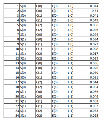
The last column in the above table represents the probability of occurrence of each of the combinations of events. Now using the above table we can answer any question related to the mentioned four variables. E.g.,

The probability of a person having lung cancer knowing that he smokes has more than 5 friends that smoke, and that he exercises regularly is 0.055. (Row 24 of the above table represents this probability). Let's consider another one.

The probability that a person has lung cancer is 0.54. (We need to sum up the probability values of the rows which state that the person has lung cancer i.e., rows 13 -24 which according to the law of total probability is essential \(∑_E∑_C∑_S(S, C, E, L(1))\)). This process is called marginalization. Here we are performing three summations to marginalize and find the probability that a person has lung cancer.

Complexity in calculating joint probabilities

So far so good. We were dealing with a small problem where we were having four variables where three of them were having a level of two and one was having a level of three. Simple Enough and we have conveniently written our probability distribution table having 24 rows.

But what if we have to marginalize over 10 variables/features each of which has 5 levels (i.e., 5 different categorical values), how many different combinations do think we need to calculate? Pause to think about it.

\(5^10\). Each variable has 5 levels and there are 10 such variables, where the number of combinations = 5 x 5 x 5 ....10 times.

We have seen that the joint probability distribution table is used to look up the probability values corresponding combination of features. Given a probability distribution over d variables and each of the variables take k different values, the size/number of rows of this joint probability distribution table will be \(k^d\).

Marginalization is a computationally expensive process to make an inference/prediction. We have seen the number of summations one needs to perform to make an inference over partial data. Therefore, we need to reduce the size of the joint probability distribution table to make it quicker.

The joint probability distribution table can be solved using some tricks such as exploiting the independencies between the variables. The total number of rows reduces drastically if all the variables are independent of each other but that is an impossible situation in a real-life scenario. Also, it is highly unlikely that none of the variables is independent of the other. 

For a probability distribution over d variables which take k different values, if all variables are independent of each other, we can write the probability distribution as a multiplication of individual probability distributions as follows:

$$p(x_1,x_2,x_3,......,x_d)=p(x_1).p(x_2).p(x_3)........p(x_d)$$

If all variables are independent then the number of rows reduces drastically to \(k.d\) as we will not be having one table but instead d different tables.

In real-time use cases, there will be some independent variables (as they follow the joint probability of independence) and some variables will not be. Hence, the key to overcoming the computation problem of joint probability distribution lies in understanding the independencies between the variables. This task is simplified to a great extent with the help of graphs that can help in figuring out such independencies.

Graphs in Probabilistic Graphical Models

The graph consists of nodes and edges, as we have briefly discussed in the prerequisite section. In PGMs, these nodes represent the variables in the system, and the edges represent the relationships between these variables.

We use graphs in PGMs because they are widely studied in mathematics, so we can use a lot of the theoretical properties of graphs, They seem like a natural way to capture dependencies/independencies between the variables, and these help in simplifying the joint probability distribution. 

NOTE: A graph and the probability distribution should be equivalent to each other in a Probabilistic Graphical Model.

There are two ways to check independence among the variables. The first one is by satisfying the independency relationship and the second way is to calculate correlation/covariance. Let's go ahead and explore both of the techniques to check independence among variables.

Checking conditional independencies

Until now, we know that to simplify the marginalization problem, there is a need for a graph that correctly represents the independencies present in the joint probability distribution. The major challenge involved while building a graph that is equivalent to a probability distribution is that we don't exactly know what the independencies are in the given tabular data. Also, there are a lot of possibilities for graphs, each having its own set of independencies.

Markov Equivalence

It states that a graph and a probability distribution are Markov equivalent if all the conditional independencies in the probability distribution are captured by the graph we build. Meaning, the conditional dependencies among the variable are captured in the graph that we are building, or vice versa.

This is again not an easy problem. Assume we have a graph with n nodes, the possible number of edges that graph can have are \(n(n-1) \over 2\), and the possible number of possible graphs will be \(2^{n(n-1) \over 2}\).

Now our problem here is to find the graph that captures all the conditional independence from the possible graphs given n nodes.

Graphs are used to model the independencies in the probability distribution. But in most cases, the probability distribution cannot be expressed as a product of total independencies but as a product of conditional independencies. 

We already know that two variables are said to be independent if:

$$p(x_1, x_2) = p(x_1).p(x_2)$$

Now, let's similarly define conditional independence. If two variables \(x_1\) and \(x_2\) are conditionally independent on \(x_3\), we can verify that using:

$$p(x_1, x_2 | x_3) = p(x_1 | x_3).p(x_2 | x_3)$$

In other words, the probability distribution of  \(x_1\) and \(x_2\) conditioned on \(x_3\) is a multiplication of the probability distribution of \(x_1\) conditioned on \(x_3\) and the probability distribution of \(x_2\) conditioned on \(x_3\).

Let us consider an example where we are given a joint probability distribution for three variables x1, x2, and x3. 

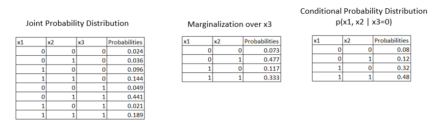
From the 1st table given above, our goal is to find if x1 and x2 are independent. To answer this we have to marginalize over x3 variables as represented in the second table above. We see that they don't satisfy the independence equation i.e., \(p(x_1=0, x_2=0) = p(x_1=0).p(x_2=0)\).

We saw that x1 and x2 are not independent but are they conditionally independent? If we condition on x3 do x1 and x2 become conditionally independent i.e., p(x1,x2|x3=0)?

Let us calculate the conditional probabilities as \(p(x1, x2 | x3=0) = {p(x1, x2, x3=0) \over p(x3=0)}\). Refer to the 3rd table which is calculated using the formula. Now we can perform the conditional independence check as,

$$P(x1 = 0, x2 = 0) = p(x1 = 0).p(x2=0)$$

which is, 0.08 = 0.2 * 0.4 = 0.08. Hence stating that variables x1 and x2 are conditionally independent.

Checking conditional independence in the graphs

The independence relationships represented by the joint probability distribution can be incorporated into a graph. And a graph is said to be Markov Equivalent to the joint probability distribution if all these independencies are captured by it.

Finding the conditional independencies from the joint probability distribution is a very difficult task and often requires domain expertise to come up with a graph structure that is Markov equivalent to the joint probability distribution. This is also an area of research and exploration happening on techniques to find a graph that is Markov equivalent to the joint probability distribution.

Let's assume the business and technical team has come up with a graph that is Markov equivalent to the joint probability distribution. How do we validate and check independencies in a graph?

Well, an edge represents the dependency between 2 nodes/variables, and hence, such independencies can be figured out. But, the real problem lies in figuring out conditional independencies.

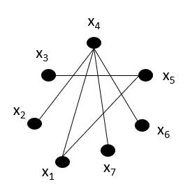
Given the graph above, \(x_3\) and  \(x_6\) are conditionally independent on which node? \(x_5\) as the only connection between \(x_3\) and \(x_6\) is via \(x_5\). Therefore, we can conclude that, in graph G, the conditional independence on a certain node 'd' occurs if the subset of nodes 'a' and 'b' become disconnected in 'G- {d}'.

NOTE: The notion of conditional independence is slightly different in directed and undirected graphs which we will be discussing later in the post.

Calculating Correlation

Let us assume some users have rated two movies M1 and M2 and we observe that ratings are correlated. The correlation here means that the user who has liked M1 has also liked M2 and the user that has disliked the movie M1 has also disliked M2.

The reason for this could be the lead actor of the movie which is the confounding factor that is not visible at first sight. But once we filter on the lead actor, now the rating of the movies is not correlated and is dependent on other factors such as the direction, and the music. It may happen that, still, most of the ratings would still be positive as we have filtered on those users who liked the lead actor.

But, do positive ratings in both columns mean that the columns are correlated? Question for thought!!!!!!

Let us take one more example dataset where variables \(x_1\) and \(x_2\) had a correlation value of 0.00001 and after conditioning on variable \(x_3\), the correlation value is 0.3. Variables \(x_1\)  and \(x_2\) are not conditionally independent on \(x_3\). As the correlation value increases upon conditioning, the variables \(x_1\) and \(x_2\) are conditionally dependent on \(x_3\). Intuitively, if two rows move in tandem, then the covariance or correlation is non zero and hence they are dependent.

At first, two columns may look correlated but when conditioned on the column they will not be correlated.

NOTE: Please note that covariance and correlation perform a similar task: check if the two variables are related to each other, but their formulae are different. Refer to the post, Confound between Covariance and Correlation? Me too. to learn in-depth about covariance and correlation.

We have come a long way and we are at the stage where we know the challenges with probability distributions, and we have figured out that we need to reduce probability distributions to smaller distributions that represent some kind of independence or conditional independence. We have also figured out that with the help of a domain expert, we need to design a graph that is Markov equivalent to the joint probability distribution.  Let's explore further the different types of graphs possible.

Different types of graphs

There are two main types of graphs used in PGMs: Directed graphs and Undirected graphs. A directed graph, also known as a digraph, is a graph where the edges have a direction, indicating a flow or causal relationship between the nodes. Directed graphs are used to represent Bayesian Networks in PGMs, where each node represents a random variable, and the edges represent the conditional dependencies between these variables.

An undirected graph, also known as a Markov random field or Markov network, is a graph where the edges do not have a direction, indicating an association or correlation between the nodes. Undirected graphs are used to represent Markov Networks in PGMs, where each node represents a random variable, and the edges represent the conditional independence relationships between these variables.

There is an important aspect to note here that the graphs used in Probabilistic Graphical Models are meant to capture pairwise interactions. The interaction between two nodes is often referred to as one node/variable influencing the other. This depends on the type of graph (i.e., directed or indirect graph) we use to represent the probability distribution.

Having an understanding of the objective behind PGMs, in the rest of the post we will be looking at how to solve PGMs for directed and undirected graphs. Let us start with understanding directed models.

Directed Graphical Models

Directed probabilistic graphical models are used extensively in the field of research and development, in the healthcare industry, and many other areas. Let us quickly understand what directed graphs are. Directed graphs consist of two things: Nodes which represent the random variables and single-headed arrows which represent the direction of influence between nodes.

A variation of directed graphs is called directed acyclic graphs (DAG). The word 'acyclic' means there should be no cycles in the graph.

Hammersley–Clifford Theorem

Hammersley-Clifford theorem provides a way to factorize the joint distribution, and this factorization eventually leads us to avoid calculating the Joint Probability Distribution (JPD) and deal with the Conditional Probability Distributions (CPDs) which are significantly cheaper to handle.

For directed graphs, the Hammersley-Clifford theorem provides a way to factor a joint probability distribution (JPD).

$$p(x_1,x_2,...,x_n)=∏^n_{i=1}p(x_i|Parents(x_i))$$

A node might or might not have a parent node. In case there is no parent, the conditional set will be empty for that node. Let us consider an example directed graph and represent the joint probability distribution using the Hammersley-Clifford theorem.

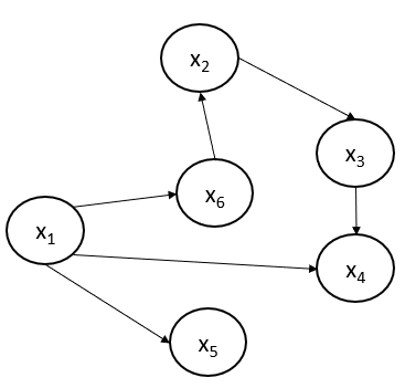
The joint probability of the acyclic-directed graph shown above can be represented using the Hammersley-Clifford theorem:

$$p(x_1,x_2,x_3,x_4,x_5,x_6) = p(x_1)×p(x_2|x_6)×p(x_3|x_2)×p(x_4|x_1,x_3)×p(x_5|x_1)×p(x_6|x_1)$$

Working with large joint distributions is computationally very expensive. By using the Hammersley-Clifford theorem, one doesn’t directly deal with the joint distribution but instead deals with the conditional probability distributions (CPDs), which are far less expensive.

Bonus: Is the Hidden Markov Model an example of a directed probabilistic graphical model?

Yes, the Hidden Markov Model (HMM) is an example of a directed probabilistic graphical model (PGM). In a directed PGM, also known as a Bayesian network, the edges in the graph represent direct causal relationships between the variables.

In an HMM, the model consists of two sets of variables: the hidden state variables and the observable output variables. The nodes represent hidden states and observable outputs, and the edges represent the causal relationships between them. Specifically, the edges in the HMM graph represent the probabilities of transitioning between hidden states and emitting observable outputs.

Understanding conditional independence in the directed graph

So far we have seen how to check if the random variables are independent or conditionally independent by checking independencies or calculating correlation. Let us now understand the independence among random variables in a directed model.

Consider a graph where we have three variables \(x_1\), \(x_2\), and \(x_3\) represented as,

$$x_1 -> x_2 -> x_3$$

We can write the joint probability distribution of the graph shown above just going by arrows as,

$$p(x_1, x_2, x_3) = p(x_1).p(x_2 | x_1).p(x_3 | x_2)$$

We can write the above factorization because of graph structure, but the default factorization will be,

$$p(x_1, x_2, x_3) = p(x_1).p(x_2 | x_1).p(x_3 | x_1,x_2)$$

In graphical terms, two variables are said to be independent of each other if they do not have a ‘direct’ edge between them (though they can be connected via an intermediate variable). In probability terms, this is equivalent to the fact that the two variables are independently conditioned on the intermediate variable, i.e. \(p(x_3 | x_2, x_1) = p(x_3 | x_2)\) implies that \(x_3\) and \(x_1\) are independently conditioned on \(x_2\).

Using a Directed Model to Make Inferences

A directed probabilistic graphical model has three parts:

1. The variables are the nodes in the graph.
2. The structure is defined by the placement of the nodes and the directed arrows.
3. The parameters are CPDs are the model parameters.

In other words, if we need to use a directed model, we need to have the variables, the graph structure, and the parameters (which are conditional probability distributions) of the model. If these three things are there then we can ask any kind of query from a directed model.

Let us consider an example directed graph as shown below. 

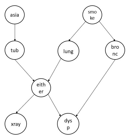
Using the Hammersley–Clifford Theorem we can write the joint probability of the above graph as:

$$p(a, t, s, l, b, e, x, d) = p(a).p(t|a).p(s).p(l|s).p(b|s).p(e|t,e).p(x|e).p(d|e,d)$$

The parameters here mean calculating the factorization of above give joint probability such as \(p(a)\), \(p(t|a)\), etc. Here every variable takes only two values yes or no. The beauty of writing the above factorization is that now we have to calculate with only 36 probabilities instead of \(2^8=256\) probabilities.

Having learned such CPDs, our task is to answer questions which means computing the probabilities of some variable(s), given some evidence. This process is also called inference. In a nutshell, computing the probabilities of a random variable given some evidence is called inference.

E.g., Considering the graph shown above, we need to calculate that the x-ray value is 1 given that the person is a smoker. To answer this question, we should be able to write the \(p(x=1 | s=1)\) in terms of the conditional probabilities that we already calculated earlier as we don't have the direct answer available.

But consider if we need to calculate a person is having lung cancer given he smokes \(p(l=1 | s=1)\. This we can calculate directly as we already know \(p(l|s)\.

There are multiple techniques that we can use to infer the results. In this post, we will be covering two of them: Variable elimination and message passing algorithm.

Let's get started.

Variable elimination

Let us consider the same example and we want to infer \(p(x=1 | s=1)\). How we will calculate this using the variable elimination technique?

Using conditional probability, we can write \(p(x=1 | s=1)\) as:

$$p(x=1 | s=1) = {p(x=1, s=1) \over p(s=1)}$$

We already know \(p(s=1)\). Therefore we need to calculate next \(p(x=1, s=1)\). We already know the law of total probability and marginalization. Therefore we can write as

$$p(x=1 , s=1) = \sum_{a, t, l, b, e, d}p(x=1, s=1, a, t, l, b, e, d)$$

And above probability can be easily factorized into the conditional probabilities that we saw earlier using Hammersley–Clifford Theorem:

$$p(x=1, s=1, a, t, l, b, e, d) = \sum_{a, t, l, b, e, d}p(a).p(t|a).p(s=1).p(l|s=1).p(b|s=1).p(e|t,e).p(x=1|e).p(d|e,d)$$

If we look at the graph, intuitively speaking nodes "asia", "bronc", and "dysp" doesn't have any impact while calculating \(p(x=1, s=1)\). Therefore, intuitively speaking we should be able to eliminate them from the above equation.

If we see the above equation, the Only terms for the node "asia" are \(p(a)\) and \(p(t | a)\). On refactoring the equation and grouping all "asia" nodes can be represented as \(\sum_a p(a).p(t, a)\) which is equivalent to \(\sum_ap(a, t)\) which is nothing but p(a). In the same way, we can eliminate nodes b and d as well. Therefore our inference reduces to

$$p(x=1, s=1, a, t, l, b, e, d) = \sum_{t, l, e}p(t).p(s=1).p(l|s=1).p(e|t,e).p(x=1|e)$$

On substituting the value in our original equation we get the below equation as \(p(s=1)\) gets canceled out with the denominator.

$$p(x=1 , s=1) = \sum_{t, l, e}p(t).p(l|s=1).p(e|t,e).p(x=1|e)$$

where \(p(t) = \sum_a p(a).p(t,a)\). Now how do we calculate the result for the above equation?

It turns out we need to put all combinations of the four variables l, t, e, and a. The following table shows the partial calculation.

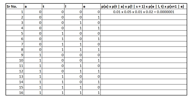
To fill the table we would need conditional probabilities, that can be calculated using the "pgmpy" Python package as demonstrated below:

# reading the file 'asia.bif' using BIFReader
from pgmpy.readwrite import BIFReader
reader = BIFReader('asia.bif')
asia_model = reader.get_model()

# print conditional probability distributions
for cpd in asia_model.get_cpds():
    print("CPD of {variable}:".format(variable=cpd.variable))
    print(cpd)

Once we have filled the column values, we need to sum them up, resulting to be 0.1517. I encourage you to solve it yourself and see if the answer is valid or not.

Using the variable elimination technique, we needed to marginalize the variables to get answer the query. It turns out that this marginalization step is computationally expensive. In the real world, there are hundreds of variables in a graph and each of them is not binary. This makes it difficult to use variable elimination in real-world problems.

Due to this limitation, numerous other algorithms are used to infer probabilities. This is still an area that is not quite mature. Researchers are working on efficient ways for inference and it is still a hard problem to find inferences in the graphical models.

One of the popular algorithms is the message-passing algorithm. This algorithm is fairly popular and can be used only for a subset of directed graphical models called rooted trees. Let's explore this next.

Message-passing algorithm

Message passing is an inference technique to get answers from a directed graphical model. It is also known by the name belief propagation. This technique can only be applied to a subset of directed graphs.

Message passing can only be applied to rooted trees. Rooted trees are the ones where every node has a single parent, and there is only one single root node for the entire tree.

Let's continue and see what is message passing.

The problem that we are going to solve is that, given some Evidence i.e. the variables for which we know the value, we need to predict the target variable.

i.e. \( p({x=1 \over E})\), here we are trying to find the probability of some node x having a certain value given certain evidence. This is what we have seen so far and this is called an inference problem which we already know. But this time we will solve this problem with a message-passing algorithm instead of a variable elimination technique.

Since the message-parsing algorithm assumes that the structure of the graph is a rooted tree. Therefore all the evidence which are given to calculate the \( p({x=1 \over E})\) can be categorized into descendants or non-descendants of x since there will be nodes that will be on top of x (non-descendants and they can be ancestors as well) and there will be nodes for which x will be a parent (descendants).

NOTE: In a tree, or directed acyclic graph (DAG), an ancestor of a node is any node that has a directed path leading to that node. In other words, any node that is a parent, grandparent, great-grandparent, and so on, of the node is considered an ancestor.

On the other hand, a non-descendant of a node is any node that is not a descendant of that node. In other words, any node that is not a child, grandchild, great-grandchild, and so on, of the node is considered a non-descendant.

Therefore the union of descendants and non-descendants of x will give us the nodes which are part of the evidence. i.e., 

$$E^x_D \bigcup E^x_N = E$$

We can rewrite, p(x|E) as,

$$p({x | E}) = {p(x, E) \over p(E)} = {p(x, E^x_D, E^x_N) \over p(E)} $$

Now \(p(x, E^x_D, E^x_N)\) can be rewritten based on the usual conditional probability:

$$p(x, E^x_D, E^x_N) = p(E^x_D | x, E^x_N) . p(x|E^x_N) =  p(E^x_D | x) . p(x|E^x_N)$$

Beauty is that \(E^x_D \)  and \(E^x_N\) are separable and can be easily calculated.

By calculating the probabilities independently for each of the evidence sets, we can imagine if each piece of evidence is giving some information to the query. This information is independent of the information given by the other evidence set. This is where the name of the message passing comes from. Each evidence set is passing, in some sense, a message.

Now let's dive deep into the technique and look at how these messages, that is, probabilities from each piece of evidence are calculated.

Let us first try to calculate \(p(E^x_D | x) \) which is equivalent to calculating all the probabilities of the descendent of x. Since all the descendent nodes (let's call then \(C_i\) ) are dependent on x and if x is removed the whole tree falls apart. Therefore, \(p(E^x_D | x) \) having k different descent nodes can be written as:

$$p(E^x_D | x) = p(E^x_{D1}, E^x_{D2} . . . E^x_{Dk} | x) = \prod^k_{i=1}p(E^x_{Di}|x)$$

Similar to what we have seen in variable elimination techniques, we will be summing up all the evidence for which the value is not provided as per the law of total probability. Therefore,

$$=\prod^k_{i=1}(\sum_{c_i} p(C_i, E^x_{Di} | x))$$

Now again based on conditional probability we can rewrite the above equation as,

$$=\prod^k_{i=1}(\sum_{c_i} p(E^x_{Di} | C_i).p(C_i|x))$$

This is how a message from one evidence set is calculated. But messages have to come from all the independent pieces of evidence. These messages come not only from the bottom of the tree but also from the top of the tree. Next, let's see how all these messages combined.

The algorithm is called the message parsing algorithm because all the dependent nodes pass the message which is \(p(E^x_{Di} | C_i).p(C_i|x)\) from \(C_i\) to x and then x node sums and multiplies all the messages it has received from the dependent nodes.

The very same process happens for the non-dependent nodes as well. There is a slight difference in parsing the messages from the non-dependent nodes to x but that is out of the scope of this post.

There have been various other versions of this same algorithm that try to generalize this and apply it to any graph, not just rooted-tree. A lot of research is still going on in the inference area of the graphical models' domain.

Types of Structures

Before studying parameter estimation and structure learning, we need to understand the different kinds of structures that are possible inside a directed graph. After all, to come up with a graph, we need to understand all the interdependencies between different variables in the graph.

There are four different types of structures possible in a directed graph. Let's explore them next.

Non-collider Structure 1 and 2

Below are the two possible non-collider structures possible in the directed graph. But what if I tell you that the below shown two structures represent the same equation according to the Hammersley-Clifford theorem?

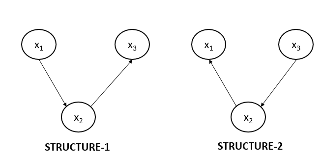
Let us write the joint probability distribution for both of the graphs shown above. For the first graph, JPD will be:

$$p(x_1, x_2, x_3)= p(x_2).p(x_2|x_1).p(x_3 | x_2)$$

And for the second graph, the JPD will be:

$$p(x_1, x_2, x_3)= p(x_3).p(x_2|x_3).p(x_1 | x_2)$$

We can rewrite the JPD of the second graph exactly as that of the first graph. Let's see how we can do this next. Using the standard rule of conditional probability we can rewrite it as:

$$p(x_1, x_2, x_3)= p(x_2, x_3).{p(x_1, x_2) \over p(x_2)}$$

Further, we can write \(p(x_2, x_3) = p(x_3 | x_2) .p(x_2)\) and \(p(x_1, x_2) = p(x_2 | x_1) .p(x_1)\). Substituting the values in the above equation we get

$$=p(x_2).p(x_2|x_1).p(x_3 | x_2)$$

which is identical to the joint probability distribution equation that we have written for the first graph above. Therefore, both the graphs shown above are equivalent.

Till now we had explored that a directed graph implies a unique relationship between the variables. But as we just saw, the two types of structures imply the same equations according to the Hammersley-Clifford theorem. So how do you disambiguate one structure from the other?

Directed graphs are a way for us to reason about real-life scenarios. For example, we know that, for an employee, the salary hike depends on their job performance. The better the bonus, the happier the employee will be. The graph of this situation can be something like the one shown in the graph below.

J -> S -> H, where, J stands for 'Job Performance', S stands for 'Salary Hike' and H stands for 'Happiness'. 

Now, going by what we just observed, the H -> S -> J also implies the same distribution as the one shown below.

For all we know, happiness can’t probably lead to a salary hike. And salary hike can’t lead to an individual performing well. If we think about it intuitively, these two are very different cases. But from the point of view of graphical models, they’re equivalent. That suggests that graphical models are not always ideal for modeling real-life scenarios. But they're one of the most effective models for causal reasoning that we know today.

Non-collider Structure 3

Now, let’s look at the third type of non-collider structure. This structure is also equivalent to the above two structures we just saw.

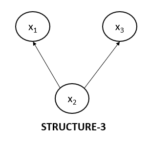
Let's write the joint probability for the above graph.

$$p(x_1, x_2, x_3)=p(x_2).p(x_1|x_2).p(x_3 | x_2)$$

Let's rearrange the equation and replace \(p(x_1 | x_2) = p(x_1, x_2) .p(x_2)\).

$$p(x_1, x_2, x_3)=p(x_1, x_2).p(x_3 | x_2) = p(x_2).p(x_1|x_2).p(x_3 | x_2)$$

Again we get the identical equation that we have got for the first graph.

Stating, all three structures that we saw are Markov equivalent. This makes it very challenging to come up with a graph that is Markov equivalent to the CPD. That is the reason why a domain expert is needed to build a graph.

Now, there’s the fourth type of structure which is not the same as the above three. Let’s look at the fourth structure and how is it different from the previous three.

Collider Structure 4

The below diagram represents the fourth collider structure, which is indeed different from the above three structures which we have discussed.

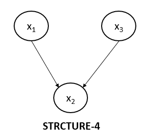
As we have done so far, let's write the joint probability for the above graph as well.

$$p(x_1, x_2, x_3)=p(x_1).p(x_3).p(x_2 | x_1, x_3)$$

Now this equation can't be written in the form of the first graph that we have seen earlier. In all the above three possible graphs there were two conditional probabilities but in this graph, there is only one conditional probability. Because of this, the equation cannot be rewritten in form of the equation of the first graph.

This is happening because in all other three graphs variables \(x_1\) and \(x_3\) were conditionally independent on \(x_2\). But here variables \(x_1\) and \(x_3\) are independent only. Let's calculate the probability \(p(x_1, x_3)\).

$$p(x_1, x_3)=\sum_{x_2}p(x_1).p(x_3).p(x_2 | x_1, x_3) = p(x_1).p(x_3)\sum_{x_2}p(x_2 | x_1, x_3)$$

The value of \(\sum_{x_2}p(x_2 | x_1, x_3) = 1\). Therefore stating the variables \(x_1\) and \(x_3\) are independent for the fourth graph structure which is not the case for the other three graph structures.

So in a nutshell, there are only two types of microstructures in a directed graphical model.

• In the non-collider structure, \(x_2\) and \(x_3\) are dependent on each other. But once we fix the value of  \(x_1\), they both become independent.
• While in the collider structure, it's the opposite. \(x_2\) and  \(x_3\) are independent of each other. But once we condition on  \(x_1\), that is once we provide the value of  \(x_1\), nodes  \(x_2\) and  \(x_3\) become dependent on each other.

Let us consider an example of the same graph that we looked at earlier.

Can we tell by looking at the graph whether the nodes ‘Asia’ and ‘lung’ are dependent or independent of each other? Or can we tell whether ‘either’ is dependent on ‘bronchitis’ or not?

The concept of d-separation will enable us to tell the independence between any two given nodes in a directed graph.

D-separation

D-separation is a critical idea in Bayesian Networks. It is used to determine whether two variables are independent of each other given a set of observed variables in a directed graph. The “d” in d-separation stands for dependence.

D-separation defines the Markov properties on directed graphs. The pairwise Markov property states that two non-neighboring variables are conditionally independent given all other variables.

Let us consider our example again and we want to check whether the variables ‘tub’ and ‘bronc’ are independent or not when ‘either’ is observed. Now, there are two paths to go from ‘tub’ to ‘bronc’. Let’s consider them separately.

NOTE: We say that a node is observed when we want to check the conditional independence between two variables A and B given the variable C. The variable C is called the observed variable.

Path 1 is tub-either-dysp-bronc. In this path, ‘either’ is observed. Therefore, ‘tub’ and ‘dysp are independent. If ‘tub’ and ‘dysp’ are independent then ‘tub’ and ‘bronc’ are also independent and therefore d-separated in this path.

Path 2 is tub-either-lung-smoke-bronc: Since ‘either’ is observed and are colliders, ‘tub’ and ‘lung’ are not independent. Now, ‘lung’ and ‘smoke’ are also not independent, and neither is ‘smoke’ and ‘bronc’ independent. Therefore, in this path, ‘tub’ can influence ‘bronc’ and they're not d-separated in this path.

So far great. Let us consider another scenario when no intermediate node is observed. This case is a simple one. There is no observed node. Suppose we want to check the dependence between ‘either’ and ‘bronc’. There are only two paths again. Let's check them separately.

Path 1 is either-dysp-bronc: This path is a colliding structure. So ‘either’ and ‘bronc’ are independent variables. Looking only at this path, the two variables are d-separated.

Path 2 is either-lung-smoke-bronc: In this path, consider the microstructure smoke-lung-either. Since it’s a non-colliding structure, ‘either’ is not independent of ‘smoke’. And ‘smoke’ and ‘bronc’ are also not independent because of the direct edge between them. Therefore, the two variables are not d-separated from this path.

For any two variables to be d-separated, they need to be independent of each other from all possible paths. Information can't flow between the two nodes because of the collider node then the variables are d-separated.

Knowing the graph structures, let's proceed forward and understand parameter estimation.

Parameter Estimation

We already know how to make use of a model and do different kinds of inferences using the model. However, the question that comes to mind is how we arrive at the model.

When we start working on a problem, we’ll only have the dataset and the different variables as the columns in the dataset. To arrive at the model, we need to find out the structure first and then the parameters of the model.

Structure learning is, however, still an open problem and even the theory is not mature at the moment to give robust enough results. We will look at structure learning later in the post.

Now, let’s see how one estimate or find the parameters, that is, all the conditional probabilities in a directed graph. It is recommended to know the maximum likelihood estimation (MLE) before proceeding forward. Refer to the post, Logistic Regression Detailed Explanation.

As we have seen earlier that in a directed graph, the joint probability can be written as the conditional probabilities of each of the individual nodes given their parents because of the Hammersley-Clifford theorem.

$$p(x_1,x_2,...,x_n)=∏^n_{i=1}p(x_i|Parents(x_i))$$

The above equation is my model, where the task is to figure out all the conditional probabilities \(p(x_i|Parents(x_i))\). To figure out these probabilities let's assume we have a dataset that has features labeled as \(x_1, x_2, x_3, . . . ., x_n\) and has m observations labeled as \(y_1, y_2, y_3, . . . ., y_m\).

Each feature in the tabular dataset represents one node. Let's assume there is a node \(x_i\) in the given graph. Given a feature \(x_i\), it will have some parent features, and in the same way \(x_i\) will be a parent feature for some other features. Hence, graphical models can encapsulate the relationships among the features.

Let's call the set of all the parents to \(x_i\) as \(P_i\). We can now write the joint probability distribution for any set of features. Consider one such data point for which we need to write the probability distribution as \(p(x_1,x_2,...,x_n)=∏^n_{i=1}p(x_i|P_i)\).

Now consider a dataset where we have m data points and consider a point \(y_{ji}\) where \(j\) represents the \(j^{th}\) data point and \(i\) represents the \(i^{th}\) column value, we can write the probability distribution of occurrence of \(j^{th}\) datapoint as all the feature values of \(j^{th}\) datapoint occurring together:

$$p(y_j) = p(y_{j1}, . . ., y_{jn}) = \prod^n_{i=1}p(y_{ji} | P_i)$$

Now the probability that the entire dataset could have occurred can be represented as the likelihood of the dataset and can be represented as the product of all the data points:

$$∏^m_{j=1}p(y_j)=∏^m_{j=1}∏^n_{i=1}p(y_{ji}|Parents(i))$$

In the above equation, 'j' represents the row index, and 'i' represents the column index.

Now that we’ve got the equation of the likelihood of the dataset, we need to find the probabilities for which the likelihood is maximized. This is a simple optimization problem to solve for.

For convenience, we will not be maximizing the likelihood equation, but we will take the log of the equation and maximize the log likelihood of the function. This is primarily done to simplify the calculation and calculate summations instead of products.

Log-likelihood of the equation is represented as:

$$\sum^m_{j=1}log(p(y_j))=\sum^m_{j=1}\sum^n_{i=1}log(p(y_{ji}|P_i))$$

We can rewrite the equation as \(=\sum^n_{i=1}[\sum^m_{j=1}log(p(y_{ji}|P_i))]\), basically just changing the order of summation. Now, for every feature x, we are calculating all the data points as:

$$p(x_i = c | p_i) ={n_{i = c} \over n_{p_i}}$$

In the above equation, we are filtering the dataset and figuring out the number of data points that are parents, and out of the filtered dataset we are looking at the number of data points for which a given feature value is c. This is very similar to what we do in the Naive Bayes algorithm.

To summarize, parameter learning is essentially given data and a graph we count for every node given the parent values, apply the filter on the parent values, and from the filtered set look at the fractions of datapoint which has specific values for the columns and ratio will be the conditional probabilities and finally we have an entire model with us.

Structure Learning

Structure learning is the hardest part of graphical models today. In most of the problems, the structure is arrived at by talking to domain experts. Take, for instance, the healthcare industry. The doctor has a great deal of knowledge about the causal effects of different symptoms on different diseases and conditions. So, when it comes to making a directed model for disease diagnosis, the graph is arrived at by consulting the doctors.

Similar is the case with other domains. Ideally, we should have an algorithm that creates a graph for us. That’s because we expect machine learning and AI to look at the hidden patterns in the data that even domain experts with all their experience can’t see. A human only is capable of looking at a small sample out of all the possible cases. That’s where ML and AI can play a significant role. We just feed all the data that was probably witnessed by thousands of doctors, and then you let the machine and algorithms decide which is the best graph, that is, what are the different causal relationships between different variables.

Today, however, we do not have such robust algorithms which can provide us results better than the industry experts. Although, still in progress, let us understand the process of structure learning.

Before we close this section, there's another popular jargon used while working with directed graphs called immoralities.

In a collider structure (a --> b <-- c), if there is no direct edge between 'a' and 'c', then immorality is said to exist between the two nodes. Immorality is just another way to let us know that there is a collider node between the nodes 'a' and 'c'.

Undirected Graphical Models

So far, we have covered directed graphical models. Let's move forward and discuss the undirected graphical models. We will see how the inference and properties of graphs change as we remove the directions from the graphs. 

Undirected graphical models are easier to model as compared to directed graphical models. The only difference in the graph structure in directed and undirected graphical models is that the edges don’t have any direction in undirected graphical models.

Please note that since undirected graphical models have a variety of applications each leading to numerous graph structures, here we will just be understanding how the concepts are fundamentally different from the directed graphical models. Examples and detailed mathematical derivations are out of the scope of this post. It can serve as a good starting point for someone who wants to dive deeper.

Hammersley-Clifford theorem for undirected graphs

We have already discussed Hammersley-Clifford theorem for the directed graphical models. Let's see how it is different for the undirected graphical models. It states that a graph and a joint probability distribution are Markov Equivalent if and only if:

$$p(x_1,x_2,...,x_n)={1\over Z} \prod^{N_c}_{i=1}ψ(x_{ij}:x{ik}∈c{i})$$

where \(N_c\) is the number of cliques, \(x_{ij}:x_{ik}\) are the nodes that belong to the clique \(c_i\), the terms ψ present in the multiplication stated by the Hammersley-Clifford theorem are potential functions associated with terms representing the maximal cliques and Z is the normalizing constant.

How to calculate Z is out of the scope of this post. But to give a brief idea, there is no need for a normalizing factor in directed graphical models because the probabilities automatically sum up to 1. Hence, Z = 1, but such normalization Z is needed in undirected graph models.

The notion of d-separation in undirected graphical models is really simple. X⊥Y|Z states that the subset of nodes X and Y are independently conditioned on Z when upon removal of Z there exists no connection between the subsets of nodes.

Clique

A clique is a part of the graph in which all the nodes or vertices are fully connected. A maximal clique has the highest number of nodes that satisfy the definition of a clique.

But why is the maximal clique important?

We have discussed earlier that more the independence is involved among the variables easier it is to model or write joint probabilities for the probabilistic graph model. Ideally, if all the variables are independent of each other we then just have to take the product of the probabilities of each variable without worrying about dependencies. And messier case is when all the variables are dependent on each other, then there is no way to decompose the problem into a somewhat simpler problem.

To factorize a joint probability for an undirected graph, we need to look for maximal cliques. The product of the potential functions of these maximal cliques will give you the joint probability (after normalizing using Z). Now, while looking for maximal cliques, we should make sure that you include every node of the graph and don't leave any of the nodes.

Let us consider an example shown below and write a joint probability distribution for it. The joint probability is represented as the product of the maximal clique.

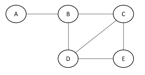
Therefore, the joint probability distribution of the above graph can be represented as a product of maximal cliques.

$$p(A,B,C,D,E)∝ψ(A,B)×ψ(B,C,D)×ψ(C,D,E)$$

NOTE: For the Hammersley-Clifford theorem to hold, no combination of the nodes should have the probability value zero. It is equivalent to removing the nodes causing the probability value to become zero and then applying the Hammersley-Clifford theorem.

Let us look again at the joint probability distribution that we have written for an undirected graph using the Hammersley-Clifford theorem. The expression of the joint probability distribution can be written by taking the log on both sides as follows:

$$log(p(x_1,x_2,...,x_n))= \sum^{N_c}_{i=1}log(ψ(x_{ij}:x{ik}∈c{i})) - log(Z)$$

The primary motivation behind taking the log is that it is harder to deal with the product than the sum. Therefore, we deal with log probabilities so that we can add them instead of taking the product.

It is visible that the log of the normalizing factor, Z has to be calculated and as discussed earlier such calculation is out of the scope of this blog. But we will look at how to use energy functions to calculate the other part: \(log(ψ(x_{ij}:x{ik}∈c{i}))\).

The transformation that we apply to tackle the problem of log values is as follows:

$$ψ(c_i)=e^{−E(c_i)}$$

The potential function is written as the negative exponential of the energy function. Upon applying this transformation, we can see that the sum of logs of potential functions becomes the sum of the energy functions with a negative sign.

$$log(p(x_1,x_2,...,x_n))= -\sum^{N_c}_{i=1}E(C_i) - log(Z)$$

Next, let us create an intuitive understanding of the energy function. We will be covering the basics of the energy function and will be discussing it in detail in an upcoming post.

Understanding the Energy Function

The energy function is used quite often in thermodynamics and can be analogized as interaction within the individuals of a colony and inter-colony interactions as interaction within a maximal clique and inter-clique interactions.

Please note that an inter-clique interaction is also a maximal clique. Hence, there is an energy function to quantify the interactions between the maximal cliques.

An energy function for any two molecules measures the discord between the pair of molecules in a thermodynamic setting. If both have the same state, the energy function has low values; if they are in different states, it will have a high value.

Such an analogy is used in the case of image segmentation where pixels act as molecules. So, if we want to segment the image into foreground and background, if a pixel and all its neighboring pixels belong to the same class, that is, foreground or background, then the energy between this pixel and its neighbors will be low.

This also means that if the neighboring pixels belong to a particular class, it is highly likely that the pixel also belongs to the same class. And we use this notion to segment a given image into the next segment.

For any two identical undirected graphs P and Q, if the energy among the two is the same, that means that the expression of the joint probability of the two graphs is also the same.

For any two different, that is, unidentical undirected graphs P and Q, if the energy among the two is the same, that means the expression of the joint probability of the two graphs may or may not be the same.

I will be writing a detailed post on Image Segmentation which will help uncover how energy functions are used in practical scenarios. Stay Tuned.

Summary

In conclusion, a probabilistic graphical model (PGMs) is a powerful algorithm for representing complex dependencies between variables. PGMs use graphical structures to encode probabilistic dependencies between variables, which can be either directed or undirected.

One of the key strengths of PGMs is their ability to represent conditional independence relationships between variables compactly and intuitively. By using graphical structures to encode these relationships, we can simplify calculations and make the models more interpretable. PGMs also provide a framework for probabilistic inference, which allows us to reason about the probability of unobserved variables given observed data. The algorithm works well even if the value of the few variables is unknown.

Overall, PGMs are a versatile and powerful tool for representing and reasoning complex dependencies between variables. As the field of data science continues to grow, PGMs are likely to become even more important and widely used in a variety of applications.