Decision Tree Detailed Explanation

Decision Tree (a tree-based algorithm) is high interpretability and an intuitive algorithm. It works almost the same as that of the human mind works for decision making. We can think of it as a nested if and else statements forming an upside-down tree.

Therefore, it is very easy to explain the results of the model to the business team.

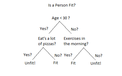
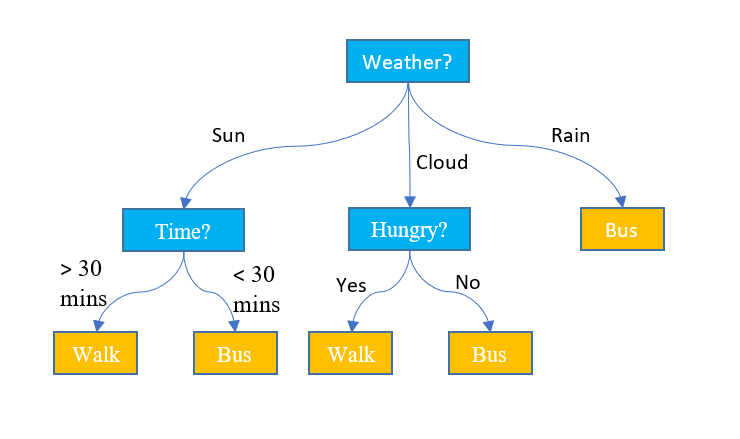
As you can see in the diagram shown above, on each node we ask the question and based on the answer we either go left or right. Also, note that the leaf of the decision tree is where the actual decision is made.

In the diagram, we are only splitting the node into two sub-nodes creating a binary decision tree. It is also possible to split the node into more than two partitions, this is called a multiway decision tree.

Regression with Decision Trees

Sometimes, we have a type of problem statement and data in such a way that we need to divide the dataset into subsets before applying linear regression.

For e.g. Predict weight of person across various ages and heights.

The difference between decision tree classification and decision tree regression is that in regression, each leaf represents a linear regression model, as opposed to a class label.

Algorithms for Decision Tree Construction

In order to construct a Decision tree, there are few learning algorithms that are used. These are:

• Homogeneity measures
  • Gini index
  • Entropy and information gain
  • Splitting by R-squared

Let's understand these learning algorithms in detail.

Homogeneity measures

Consider a scenario where we have a lot of features, how to decide the first feature on which we need to split the data? (Should it be a random selection or there should be some criteria to decide the node for the first split?)

It depends on the homogeneity of the feature. We try to split the data on the feature and check the homogeneity of the data. We do this on each and every feature and compare the homogeneity. The feature having the highest homogeneity is the feature we will be splitting data first.

Our goal is to have high homogeneity, so we keep on doing the split on every node such that homogeneity increases. We define a threshold using which we determine the stopping point for the further split. If homogeneity > threshold we stop the further split. 

We have an understanding that we need to maximize the homogeneity, but how to measure the homogeneity? There are various ways to quantify/measure homogeneity, such as:

• Gini index
• Information gain
• Entropy
• R Squared

Let's understand in the detail.

Gini index

The Gini index is represented as:

$$Gini Index = \sum_{i=1}^kp_i^2$$

where \( p_i\) is the probability of finding a point with the label i, and k is the number of different labels.

Consider an example shown below, where we have two features Gender and Age. And we need to find whether the applicant will be provided with a loan or not. The summation result of historical data is given below:

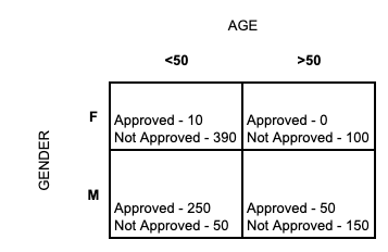
We have 1000 loan applicants in our system.

Now our goal is to find, out of two on which feature should we split first so that we have high homogeneity? Let's find the Gini Index if split on Gender and Age:

$$Gini Index (Gender) = {[{500 \over 1000}]} * {[({10 \over 500})^2 + ({490 \over 500})^2]} + {[{500 \over 1000}]} * {[({300 \over 500})^2 + ({200 \over 500})^2]} = 0.74 $$

$$Gini Index (Age) = {[{700 \over 1000}]} * {[({260 \over 700})^2 + ({440 \over 700})^2]} + {[{300 \over 1000}]} * {[({50 \over 300})^2 + ({250 \over 300})^2]} = 0.59 $$

Higher the Gini Index higher the homogeneity. Therefore we choose the feature with a higher Gini Index. Hence we will choose Gender attribute in above example.

Or in other words, Splitting on gender is expected to be more informative than age.

Entropy and Information Gain

Entropy is the measure of disorderness and is represented as: 

$$\epsilon[D] = \sum_{i=1}^kP_ilog_2P_i$$

where \( p_i\) is the probability of finding a point with the label i, k is the number of different labels, and ε[D] is the entropy of the data set D.

NOTE: Lesser the disorder, lower the entropy, greater the homogeneity and greater the Gini Index. (i.e. If a data set is completely homogenous, then the entropy of such a data set is 0)

And Information gain is the measure of how much the entropy has decreased between the parent set and the partitions obtained after splitting. Information gain is represented as:

$$Gain(D,A) = \epsilon[D] - \epsilon[D_A] = \epsilon[D] - \sum_{i=1}^k(({|D_{A=i}|\over|D|})\epsilon[D_{A=i}])$$

where ε[D] is the entropy of the parent set D (data before splitting), \( \epsilon[D_A]\) is the entropy of the partitions obtained after splitting on attribute A, \( \epsilon[D_{A=i}]\) is the entropy of the partition where the value of attribute A for the data points is i,  \( D_{A=i}\) is the number of data points for which the value of attribute A is i, and k is the number of different labels.

NOTE: The information gain is equal to the entropy change from the parent set to the partitions. So it is maximum when the entropy of the parent set minus the entropy of the partitions is maximum.

Let's consider the same example of a loan applicant:

The entropy of the dataset is given as:

$$Entropy = {-({300 \over 1000})} * \log_2({310 \over 1000}) {-({690 \over 1000})} * \log_2({690 \over 1000}) = 0.89317$$

The entropy if we split dataset on gender is:

$$Entropy (Gender) = 0.5 * [{-({10 \over 500})} * \log_2({10 \over 500}) {-({490 \over 500})} * \log_2({490 \over 500})] + 0.5 * [{-({300 \over 500})} * \log_2({300 \over 500}) {-({200 \over 500})} * \log_2({200 \over 500})] = 0.5562$$

The entropy if we split dataset on age is:

$$Entropy (Age) = 0.7 * [{-({260 \over 700})} * \log_2({260 \over 700}) {-({440 \over 700})} * \log_2({440 \over 700})] + 0.3 * [{-({50 \over 300})} * \log_2({50 \over 300}) {-({250 \over 300})} * \log_2({250 \over 300})] = 0.861241$$

And Information Gain is calculated as:

• Entropy of original data set - entropy of partitions obtained after splitting on ‘gender’ = 0.89317 - 0.5562 = 0.33697
• Entropy of original data set - entropy of partitions obtained after splitting on ‘age’ = 0.89317 - 0.861241 = 0.031929

We split on the attribute that maximises the information gain. The information gain on gender is greater than the information gain on age. Therefore we split on gender.

Splitting by R-squared

So far we have seen methods to split the data into nodes for discrete target variables. But how to create a decision tree for continuous variables?

We calculate the \( R^2\) of data sets (before and after splitting) in a similar manner to what you do for linear regression models. We split the data on a feature and calculate R squared of the partitions obtained after splitting. If the R squared is greater than that of the original or parent data set we accept the split.

We keep on doing the split until we reach the threshold of acceptable R squared.

Truncation and Pruning

Decision trees tend to overfit the data. If allowed to grow with no check on its complexity, a tree will keep splitting till it has correctly classified (or rather, mugged up) all the data points in the training set. And this needs to be addressed.

We have two different techniques to deal with overfitting. These are Truncation and Pruning.

Truncation

It stops the tree while it is still growing so that it may not end up with leaves containing very few data points. Truncation is also known as pre-pruning.

There are various methods that can be used to control the size of the tree or Truncation. Some of the methods are:

• Limit the minimum size of the partition after the split: We can limit the number of data that a leaf should have to split.
• Minimize change in the measure of homogeneity: If homogeneity measure doesn't change a lot we don't split further.
• Limit the depth of the tree
• Set a minimum threshold on the number of samples that appears in the leaf
• Set the limit on the maximum number of leaves present in the tree.

Pruning

Let the tree grow to any complexity. Then, cut the branches of the tree in a bottom-up fashion, starting from the leaves. It is more common to use pruning strategies to avoid overfitting in practical implementations.

Chopping off the tree branches results in a decrease in tree complexity. And definitely helps to overcome overfitting. But how to decide if a branch should be pruned or not?

We divide the dataset into three parts, Training, Validation and Test dataset. We prune the model and calculate the accuracy before pruning and after pruning. If the accuracy of the pruned tree is higher than the accuracy of the original tree on the validation set, then we keep that branch chopped.

NOTE: After pruning, a new leaf will be assigned a label as that of one having more number of data points in its belonging majority class.

Advantages of Decision Tree

• Predictions made by a decision tree are easily interpretable.
• A decision tree does not assume anything specific about the nature of the attributes in a data set. It can seamlessly handle all kinds of data — numeric, categorical, strings, Boolean, and so on.
• It does not require normalization since it has to only compare the values within an attribute.
• Decision trees often give us an idea of the relative importance of the explanatory attributes that are used for prediction.

Disadvantages of Decision Tree

• Decision trees tend to overfit the data.
• Decision trees tend to be very unstable, which is an implication of overfitting. A few changes in the data can change a tree considerably.

Sklearn Implementation

We use the sklearn package DecisionTreeClassifier to generate a classifier model using the Decision Tree algorithm. There are few hyperparameters that need to be tunned some of them are:

1. max_depth -  the max_depth parameter denotes the maximum depth of the tree. By default, it takes “None” value.
2. min_samples_split - It tells the minimum no. of samples required to split an internal node. Default - 2
3. criterion - gini/entropy or IG
4. min_samples_leaf - It tells the minimum number of samples required to be at a leaf node. By default, it takes “1” as a value.

Let's see a demo to construct Decision Tree using the sklearn package:

import pandas as pd
import numpy as np
import matplotlib.pyplot as plt
import seaborn as sns
from sklearn.datasets import load_wine
from sklearn.tree import DecisionTreeClassifier

data = load_wine()
X = data.data
y = data.target

# You can try with changing the hyperparameter or adding new one
dt_default = DecisionTreeClassifier(max_depth=3)
dt_default.fit(X, y)

# Importing required packages for visualization
from IPython.display import Image  
from sklearn.externals.six import StringIO  
from sklearn.tree import export_graphviz
import pydotplus, graphviz

# Putting features
features = list(bunch.feature_names[0:])

dot_data = StringIO()  
export_graphviz(dt_default, out_file=dot_data,
                feature_names=features, filled=True,rounded=True)

graph = pydotplus.graph_from_dot_data(dot_data.getvalue())  
graph.write_pdf("dt_wine.pdf")

OUTPUT:

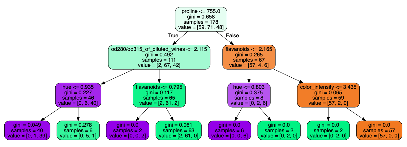
The output states that the most important feature is proline having 0.658 Gini Index.

NOTE: We should avoid creating dummy variables using one-hot encoding and instead use label encoding to convert categorical variables to numeric for decision tree. As in the case of tree-based models, 1,2,3 doesn't mean 3 is more than 1. It’s just the label that we are dividing it into.

Summary

In this post, we saw that unlike other algorithms such as logistic regression or SVMs, decision trees do not find a linear relationship between the independent and the target variable. Rather, they can be used to model highly nonlinear data. We saw the learning algorithm used to construct the decision tree:

• Homogeneity measures
  • Gini index
  • Entropy and information gain
  • Splitting by R-squared

We saw the advantages and limitations of the Decision tree. And after getting familiar with the concepts we did hands-on where we build the Decision tree.