Confound between Covariance and Correlation? Me too.

There are two key concepts: Covariance and Correlation in the statistics, but what are they about? Most importantly are they the same or do they have any differences? Are they related to each other? What are the different types of correlations?

The above are the questions that I was having initially when I started learning about statistics. In this post, I have made an attempt to answer the above-stated questions. Let's go straight into it and try to understand Covariance and Correlation.

Covariance

Let's begin by defining what covariance is. It is a measure of how two quantities vary together. We can see covariance by plotting two measures in which we need to find the relation.

Covariance answers a few of the questions like:

1. If the value of one series goes up what happens to the value of other series?
2. If the value of one series goes down what happens to the value of other series?
3. If the value of one series remains constant what happens to the value of the other series?

NOTE: If two variable doesnt show any relationship that means there covariance is near to zero. We can use scatter plots to validate the information.

Plotting a scatter plot to understand the covariance

Numpy provides function \(np.cov()\)  that accepts two datasets as an argument and returns the covariance between them. Function return 2-D array where entries [0,1] and [1,0] are the covariance. Entry [0,0] and [1,1] are covariance of the first and second datasets respectively. The 2-D array returned is also called the covariance matrix.

Consider an example shown below:

versicolor_petal_length = np.array([4.7,  4.5,  4.9,  4.,  4.6,  4.5,  4.7,  3.3,  4.6,  3.9,  3.5,
                                    4.2,  4.,  4.7,  3.6,  4.4,  4.5,  4.1,  4.5,  3.9,  4.8,  4.,
                                    4.9,  4.7,  4.3,  4.4,  4.8,  5.,  4.5,  3.5,  3.8,  3.7,  3.9,
                                    5.1,  4.5,  4.5,  4.7,  4.4,  4.1,  4.,  4.4,  4.6,  4.,  3.3,
                                    4.2,  4.2,  4.2,  4.3,  3.,  4.1])

versicolor_petal_width = np.array([1.4,  1.5,  1.5,  1.3,  1.5,  1.3,  1.6,  1.,  1.3,  1.4,  1.,
                                   1.5,  1.,  1.4,  1.3,  1.4,  1.5,  1.,  1.5,  1.1,  1.8,  1.3,
                                   1.5,  1.2,  1.3,  1.4,  1.4,  1.7,  1.5,  1.,  1.1,  1.,  1.2,
                                   1.6,  1.5,  1.6,  1.5,  1.3,  1.3,  1.3,  1.2,  1.4,  1.2,  1.,
                                   1.3,  1.2,  1.3,  1.3,  1.1,  1.3])

# Compute the covariance matrix: covariance_matrix
covariance_matrix = np.cov(versicolor_petal_length, versicolor_petal_width)

# Print covariance matrix
print(covariance_matrix)

# Extract covariance of length and width of petals: petal_cov
petal_cov = covariance_matrix[0,1]

# Output
# [[0.22081633 0.07310204]
# [0.07310204 0.03910612]]

Correlation

Correlation is the same as covariance. Let's see the difference between the two:

1. Covariance just tells us about the direction (+,-,0) between two variables. Whereas correlation tells us about direction and strength.
2. Covariance can be any number it's just the sign that we consider. But correlation is always between +1 and -1. Also, correlation is independent of the measure. We can compare the relationship between two separate measures (which are measured in different units)

NOTE: Correlation is only applicable to linear relationships. Is is recommended to plot scatter chart before finding the correlation.

Let's see scatter plots to understand the intuitiveness of the concept of correlation.

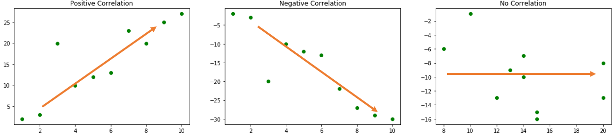
The above diagram shows three different types of correlations:

• Positive Correlation: When one variable's value increases on the increase of correlated variables.
• Negative Correlation: When one variable's value decreases on the increase of correlated variables.
• No Correlation: When there is no relationship between the variables.

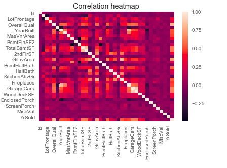
We can also plot a heatmap to represent the correlation between the dataset.

There are in general four different types of correlation in statistics:

1. Pearson correlation
2. Kendall rank correlation
3. Spearman correlation
4. Point-Biserial correlation

Let's understand them next.

Pearson correlation

Person correlation is applicable when there is a linear relationship between the variables. It's formula in terms of covariance is

$$covariance(x,y)\over {std(x) * std(y)}$$

Or in other terms,

$$r = {{\sum(x_i - \bar{x})(y_i - \bar{y})} \over {\sqrt{\sum(x_i - \bar{x})^2 \sum{(y_i - \bar{y})^2}}}}$$

where \(\bar{x}\) and \(\bar{y}\) are the mean of two variables for which we want to check the correlation.

Let's look at an example to compute the person correlation.

Similar to np.cov() function numpy provides np.corrcoef() function to calculate correlation. It accepts two datasets and returns a 2D array.

Consider an example shown below:

def pearson_r(x, y):
    """Compute Pearson correlation coefficient between two arrays."""
    # Compute correlation matrix: corr_mat
    corr_mat = np.corrcoef(x,y)
    # Return entry [0,1]
    return corr_mat[0,1]
# Compute Pearson correlation coefficient for I. versicolor: r
r = pearson_r(versicolor_petal_length, versicolor_petal_width)
# Print the result
print(r)

Spearman correlation

Spearman’s correlation is the most common alternative to the Pearson correlation. It is also named "Spearman’s Rank-Order Correlation" which is applied in the cases of the lack of normally distributed nature within the variable set.

Spearman correlation can also be expressed in terms of covariance. Here we use an additional rank function to compute Spearman correlation.

$$covariance(rank(x), rank(y))\over {std(rank(x)) * std(rank(y))}$$

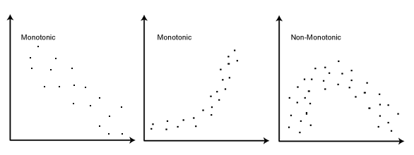
While the Pearson correlation coefficient measures the linearity of relationships, the Spearman correlation coefficient measures the monotonicity of relationships. What is the difference between linearity and monotonicity?

In a linear relationship, each variable changes in one direction at the same rate throughout the data range. In a monotonic relationship, each variable also always changes in only one direction but not necessarily at the same rate. Below are some examples of monotonic relationships.

Let's look at an example in Python to compute the Spearman correlation.

x_simple = pd.DataFrame([(-2,4),(-1,1),(0,3),(1,2),(2,0)],
                        columns=["X","Y"])
corr_s = x_simple.corr(method="spearman")
print(corr_s)

We can also use functions from the scipy package to compute Spearman correlation.

from numpy.random import rand, seed
from scipy.stats import spearmanr
# Seed random number generator
seed(1)

# Prepare data
var_1 = rand(1000) * 20
var_2 = var_1 + (rand(1000) * 10)

# Calculate Spearman's correlation
coef, p = spearmanr(var_1, var_2)
print('Spearmans correlation coefficient: %.3f' % coef)

Kendall rank correlation

Also commonly known as "Kendall’s tau coefficient". Kendall rank correlation is a measure of relationships between columns of ranked data.

Kendall rank correlation (non-parametric) is an alternative to Pearson’s correlation (parametric) when the data you’re working with has failed one or more assumptions of the test. This is also the best alternative to Spearman correlation (non-parametric) when your sample size is small.

NOTE: Parametric tests assume underlying statistical distributions in the data. Whereas non-parametric test don't rely on any distribution i.e such test can be performed regardless of the assumed distribution of data.

Kendall rank correlation formula is

$$C - D \over {C + D}$$

where C is the total number of concordant pairs and D is the number of discordant pairs. The calculations are out of the scope of this post.

Let's understand what concordant pair and discordant pairs mean.

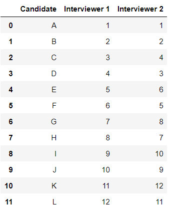
Consider an example shown above. The above example shows the ranking for different candidates from two interviewers. There are three possible scenarios in terms of ranking:

• Tied pairs: Both interviews give the same ranking to the candidate. For e.g. Candidate A.
   
• Concordant pairs: Ranking is not the same but both interviewers rank both applicants in the same order. For e.g. Interviewer 1 ranked F as 6th and G as 7th, while interviewer 2 ranked F as 5th and G as 8th. F and G are concordant because F was consistently ranked higher than G.
   
• Discordant pairs: Candidates E and F are discordant. The reason they are discordant is that the interviewers ranked them in opposite directions. For e.g. one interviewer said E had a higher rank than F, while the other interviewer said F ranked higher than E.

Several version of tau exists. The primary versions are:

• Tau-A and Tau-B are usually used for square tables (which have equal columns and rows). Tau-B will adjust for tied ranks.
• Tau-C is usually used for rectangular tables.

NOTE: Most statistical packages have Tau-B built-in.

Let's see how to calculate the Kendall correlation in python.

import pandas as pd
from numpy.random import rand
from numpy.random import seed

# Seed random number generator
seed(1)

# Prepare data
var_1 = rand(1000) * 20
var_2 = var_1 + (rand(1000) * 10)

df = pd.DataFrame({'x':var_1, 'y':var_2})
corr = df.corr(method='kendall')

There is another method as well using the scipy package.

# Calculate the kendall's correlation between two variables
from scipy.stats import kendalltau

# Calculate kendall's correlation
coef, p = kendalltau(var_1, var_2)
print('Kendall correlation coefficient: %.3f' % coef)

NOTE: Panda's data frame only supports Pearson, Kendall, and Spearman correlations.

Point-Biserial correlation

The point biserial correlation is a special case of Pearson’s correlation coefficient. It measures the relationship between the continuous and binary variables.

$${M_1 - M_0 \over s_n}\sqrt{pq}$$

where,

• \(M_1\) and \(M_0\) are the means of the group that received positive and negative binary variables respectively. 
• \(s_n\) is the standard deviation of the entire dataset
• p and q are the portion of the cases with 0 and 1 groups respectively

NOTE: Correlation doesn't mean causation.

from scipy import stats
a = np.array([0, 0, 0, 1, 1, 1, 1])
b = np.arange(7)
stats.pointbiserialr(a, b)

Bonus Point

Then what is the difference between correlation and causation?

Let me talk about a famous customer complaint. I have twisted the story to help you think and solve the puzzle. One of the customers filled a complaint at ford headquarters that his car won’t start whenever he buys vanilla ice cream and if he buys any other ice cream his car works fine.

What is happening, is there a correlation between buying vanilla ice cream and a car not getting started? Think carefully before reading further.

From the first look, it sounds that YES. Next, the technician from ford started gathering the data like time of visit, duration spent in-store, type of gas used, etc. And data showed that buying vanilla ice cream took less time than buying any other flavor as vanilla was one of the popular flavors and placed on a different shelf.

Does your observation change now? Do you still think that there is a correlation? Continue reading further.

After careful examination, it looked like the car was having an issue that it need time to cool down before getting started again. And since vanilla ice cream took less time, therefore the car didn't get time to cool down, therefore it didn't start.

In this case study, it was not vanilla ice cream. Vanilla ice cream was causation here but the actual correlation was between the time and car.

Do you know any other such real-world examples? Let's discuss them in the comment section below.