A complete guide to the Probability Distribution

We all are aware that probability is a measure of the likelihood of an event occurring in the experiment. The value of probability ranges between 0 indicating a less probable event and 1 indicating the event being the most probable.

In our post, Does probability really help businesses? we discussed how statistics can help us in solving problems and helping us to make profitable decisions. Next, let's talk about how probability distribution can help us in further demystifying the statistics.

Probability Distribution

In real-world examples, most of the problems that you will encounter will have this issue where we will have a sample dataset created by conducting experiments. So the question that you need to answer is: The sample that is collected is a true picture of the population or not?

The best way to solve this problem is to grab a paper and pen and find the probability without conducting the experiment. This is where probability distribution helps.

Probability Distribution is any form of representation that tells us the probability for all possible values of X (random variable). There are various distributions defined to generate sample data similar to the population dataset.

The type of probability distribution to be used depends upon whether the variable contains discrete values or continuous values.

A discrete distribution can only take a limited set of values i.e. Only categorical values. For. e.g. Probability of getting no of heads when we toss a coin. And continuous distributions can take in any value within the specified range. For e.g. The length of a line (can be infinite), the weight of students.

There are different types of distributions for the continuous and discrete data based on the properties of the random variable. Let us start looking at different types of continuous distributions.

Continuous Distribution

Continuous distribution can be used where the random variable is continuous. Let's see the different types of distributions that we can leverage:

• Continuous Uniform Distribution
• Normal Distribution or Gaussian Distribution
• T – Distribution
• Chi-Square Distribution
• Exponential Distribution
• Logistic Distribution

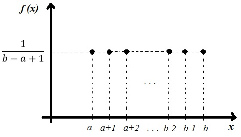
Continuous Uniform Distribution

It indicates that the probability distribution is uniform between the specified range. It is also called a rectangular distribution due to the shape it takes when plotted on a graph.

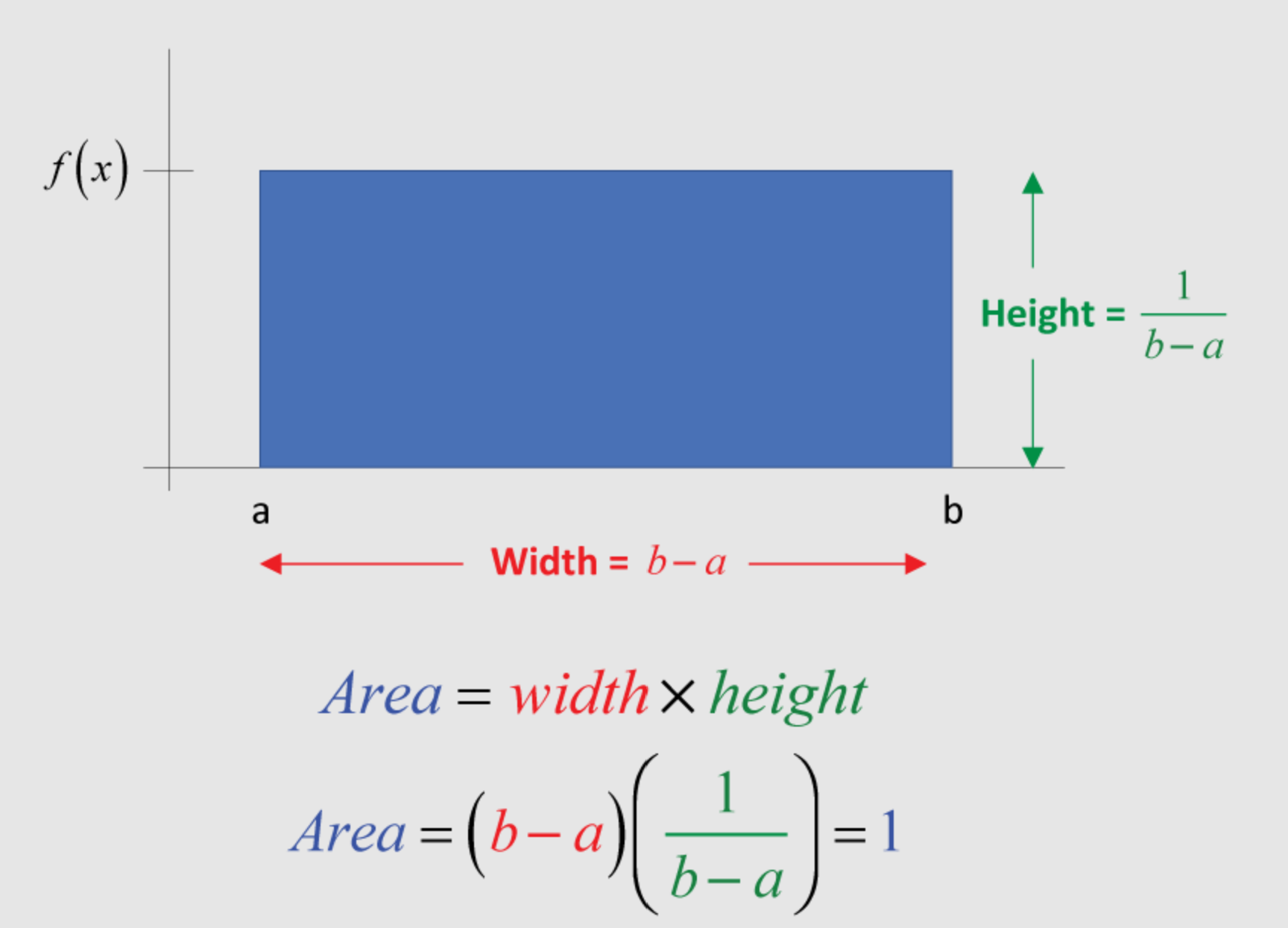
As shown in the diagram above, for a uniform distribution, \(f(x)\) is constant over the values of x.

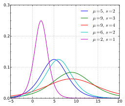
Normal Distribution or Gaussian Distribution

The Normal distribution has a single peak where the mean decides the height of the peak and the standard deviation decides the width of the curve.

It has a bell-shaped curve.

NOTE: It's best to use normal distribution if dataset doesn't have extreme outliers. If your data has a huge standard deviation, I would suggest to rethink of choice to use Normal Distribution.

Let's look at an example and use \(np.random.normal(m, s, size)\) where 

• m = mean of the data
• s = standard deviation of the data
• size = number of times the experiment will run

to sample the results from the normally distributed data. 

import numpy as np
import matplotlib.pyplot as plt

belmont_no_outliers = np.array([148.51, 146.65, 148.52, 150.7 , 150.42, 150.88, 151.57, 147.54,
       149.65, 148.74, 147.86, 148.75, 147.5 , 148.26, 149.71, 146.56,
       151.19, 147.88, 149.16, 148.82, 148.96, 152.02, 146.82, 149.97,
       146.13, 148.1 , 147.2 , 146.  , 146.4 , 148.2 , 149.8 , 147.  ,
       147.2 , 147.8 , 148.2 , 149.  , 149.8 , 148.6 , 146.8 , 149.6 ,
       149.  , 148.2 , 149.2 , 148.  , 150.4 , 148.8 , 147.2 , 148.8 ,
       149.6 , 148.4 , 148.4 , 150.2 , 148.8 , 149.2 , 149.2 , 148.4 ,
       150.2 , 146.6 , 149.8 , 149.  , 150.8 , 148.6 , 150.2 , 149.  ,
       148.6 , 150.2 , 148.2 , 149.4 , 150.8 , 150.2 , 152.2 , 148.2 ,
       149.2 , 151.  , 149.6 , 149.6 , 149.4 , 148.6 , 150.  , 150.6 ,
       149.2 , 152.6 , 152.8 , 149.6 , 151.6 , 152.8 , 153.2 , 152.4 ,
       152.2 ])

def ecdf(data):
    """ Compute ECDF """
    x = np.sort(data)
    n = x.size
    y = np.arange(1, n+1) / n
    return(x,y)

# Compute mean and standard deviation: mu, sigma
mu = np.mean(belmont_no_outliers)
sigma = np.std(belmont_no_outliers)


# Sample out of a normal distribution with this mu and sigma: samples
samples = np.random.normal(mu, sigma, size=10000)

# Get the CDF of the samples and of the data
x_theor, y_theor = ecdf(samples)
x, y = ecdf(belmont_no_outliers)

# Plot the CDFs and show the plot
_ = plt.plot(x_theor, y_theor)
_ = plt.plot(x, y, marker='.', linestyle='none')
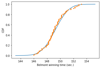
_ = plt.xlabel('Belmont winning time (sec.)')
_ = plt.ylabel('CDF')
plt.show()

Output:

The empirical rules that show the spread of the data if it follows normal distribution is as follows:

• 68% probability that the random variable falls within 1 standard deviation of the mean.
• 95% probability that the random variable falls within 2 standard deviations of the mean.
• 99.7% probability that the random variable falls within 3 standard deviations of the mean.

Let's prove it with the help of the Belmont example we have seen earlier where is data is normally distributed.

sns.distplot(belmont_no_outliers)
plt.axvline(x=mu - sigma, color='k', linestyle='--')
plt.axvline(x=mu + sigma, color='k', linestyle='--')

plt.axvline(x=mu - (2 * sigma), color='b', linestyle='--')
plt.axvline(x=mu + (2 * sigma), color='b', linestyle='--')

plt.axvline(x=mu - (3 * sigma), color='g', linestyle='--')
plt.axvline(x=mu + (3 * sigma), color='g', linestyle='--')
plt.title('1,2 and 3 standard deviation of the data')
plt.show()


data_1std = [time for time in belmont_no_outliers if time >= mu - sigma and time <= mu + sigma]
len(data_1std) / len(belmont_no_outliers) * 100        # 71.42857142857143

data_2std = [time for time in belmont_no_outliers if time >= mu - (2 * sigma) and time <= mu + (2 * sigma)]
len(data_2std) / len(belmont_no_outliers) * 100        # 94.5054945054945

data_3std = [time for time in belmont_no_outliers if time >= mu - (3 * sigma) and time <= mu + (3 * sigma)]
len(data_3std) / len(belmont_no_outliers) * 100        # 100.0

Output

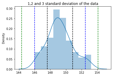
The example gave approx about 71% of data falling within one standard deviation, 94% data falling within two standard deviations, and 100% data falling within three standard deviations, justifying the empirical rules.

T – Distribution

It is similar to a normal distribution, but it has a higher probability towards the extreme values of the data.

It is preferred when the number of samples is smaller in size. With the increase in the size of samples, the t-distribution curve starts to appear like a normal distribution curve.

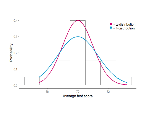
NOTE: The standard normal (or z-distribution) is the special case of the normal distribution. In standard normal distribution we have mean as 0 and standard deviation as 1.

Chi-Square Distribution

The chi-square distribution (also chi-squared or χ -distribution) with k degrees of freedom is the distribution of a sum of the squares of k independent standard normal random variables (remember standard normal distribution is a distribution with mean as 0 and standard deviation as 1).

Let say variable X represents the standard normally distributed variable, and if we take a sample from the X, then

\(Q = X^2\), where Q is the Chi-Square or Chi-Squared distribution.

Now here we are taking only one standard normally distributed variable, therefore the degree of freedom, in this case, is 1. Therefore we can write it as

$$Q \approx \chi^2_1$$

If we have two standard normal distributed variables, then \(Q = X^2_1 + X^2_2\) will be represented as

$$Q \approx \chi^2_2$$

This distribution is widely used in calculating the confidence intervals and in hypothesis testing.

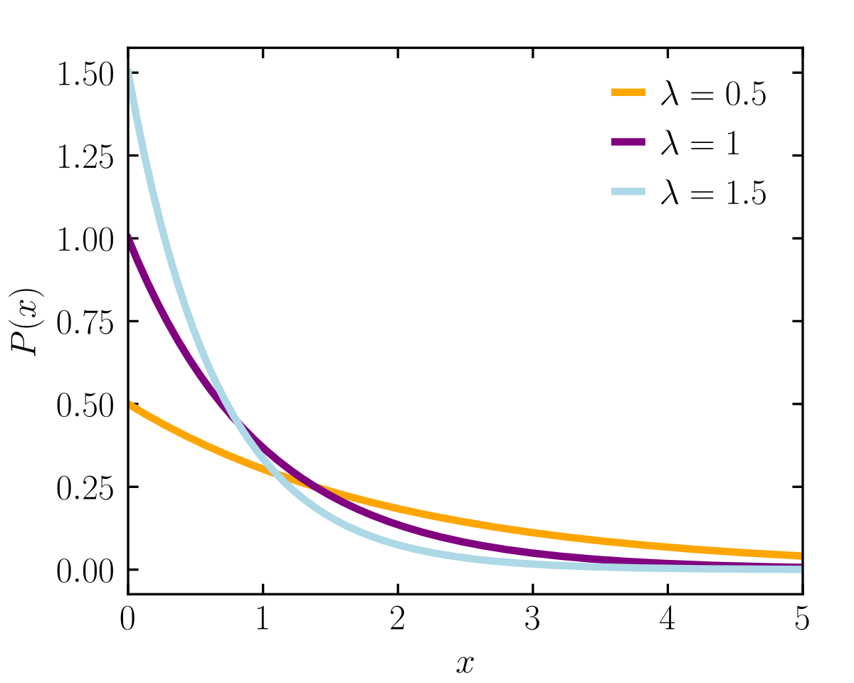
Exponential Distribution

The waiting time between the arrivals of the Poisson process is exponentially distributed. The Exponential distribution describes the waiting times between rare events. The equation for the exponential distribution is represented as:

$$y = \lambda e^{-\lambda x}$$

,which can be solved in numpy library using \(t_1 = np.random.exponential(tau_1, size)\).

NOTE: Lambda is the "rate" parameter and is proportional to how quick events are happening. If we assign lambda = 1 then we creating a distribution of event happening on average, every second, lambda = 2 means distribution of event happening on average, every two seconds and so on.

Let's assume I have collected data about how much time passed between views of this blog post.

Therefore,

\(x_1\) = the amount of time passed between 1st and 2nd blog views.

\(x_2\) = the amount of time passed between 2nd and 3rd blog views.

and so on.....

The data points collected are expected to be exponentially distributed.

Logistic Distribution

The logistic distribution is used for modeling growth and is also used in Logistic Regression. It is symmetrical distribution, unimodal (it has one peak), and is similar in shape to the normal distribution. In fact, the logistic and normal distributions are so close in shape (although the logistic tends to have slightly fatter tails) that for most applications it’s impossible to tell one from the other.

As we have explored continuous distribution, now let's explore the different types of discrete distribution.

Discrete Distribution

Discrete distribution can be used where the random variable is categorical. Let's see the different types of distributions that we can leverage:

• Binomial Distribution
• Multinomial Distribution
• Bernoulli's Distribution
• Negative Binomial Distribution
• Geometric Distribution
• Hypergeometric Distribution
• Poisson Distribution
• Discrete Uniform Distribution

Bernoulli's Distribution

This distribution is generated when we perform an experiment and the experiment has only two possible outcomes – success and failure. The trials of this type are called Bernoulli trials. Let us assume that, p is the probability of success then 1 – p is will be the probability of failure, summing up the total probability to 1.

Example of a coin toss, where the possible outcomes are either heads or tails.

Binomial Distribution

 A binomial experiment is a statistical experiment that has the following properties:

1. The experiment consists of n repeated trials.
2. Each trial can result in just two possible outcomes. We call one of these outcomes a success and the other, a failure.
3. The probability of success, denoted by P, is the same on every trial.
4. The trials are independent; that is, the outcome of one trial does not affect the outcome of other trials.

Let's consider our game at casino XYZ, where at any stage of an experiment a participant can draw either a red ball or blue ball. Therefore satisfying the properties of the binomial distribution.

Let's generalize our experiment of drawing balls from a bag. If we repeat the experiment n times with the probability p of drawing r red balls from the bag. The probability will be denoted as

$$P(X=r)={^nC_r}(p)^r(1−p)^{n−r}$$

where n is no. of trials, p is the probability of success, and r is no. of successes after n trials. And the number of combinations in which we could draw r red balls is \({^nC_r}\).

Doesn't it sound similar to the Bernoulli distribution?

Bernoulli is used when the outcome of the event is required for only one time and binomial is used when an outcome of an event is required multiple times.

In our coin flip example, if we only need to perform the experiment of coin-flipping once then it will fall under Bernoulli's distribution but we need to perform the experiment 5 times then it will fall under binomial distribution.

The above formula is also a generalized formula to calculate binomial distribution. We can calculate the Binomial distribution using the binomial function from the numpy library in python as follows:

np.random.binomial(n, p, size) where,

• n = number of trials
• p = probability event of interest occurs on any one trial
• size = number of times the experiment is ran

Let's look at an example:

# Take 10,000 samples out of the binomial distribution: n_defaults
n_defaults = np.random.binomial(n=100, p=0.05, size=10000)
# Compute CDF: x, y
x, y = ecdf(n_defaults)
# Plot the CDF with axis labels
plt.xlabel('deafuls')
plt.ylabel('deafuls')
plt.plot(x,y, marker='.', linestyle='none')
# Show the plot
plt.show()

Examples where we can use binomial distributions:

• Tossing a coin 20 times to see how many tails occur
• Asking 200 randomly selected people if they are older than 21 or not
• Drawing 4 red balls from a bag, putting each ball back after drawing it

We cannot use binomial distribution for the experiment of "Tossing a coin until a head occurs" as we don't have the number of experiments fixed here.

 Poisson Distribution

The Poisson distribution, like the binomial, is a counted number of times some event happens and is independent of one another. The difference is that:

1. With a binomial distribution, we have a certain number (n) of "attempts," each of which has the probability of success p. With a Poisson distribution, you essentially have infinite attempts, with an infinitesimal chance of success.
    
2. The Poisson distribution provides the probability of an event occurring a certain number of times in a specific period of time. For e.g: The number of views this post will receive in the next hour. We can provide probability by looking at historical data of average views per blog post, but cannot tell the exact count.
3. The binomial distribution is one, whose possible number of outcomes are two, i.e. success or failure. On the other hand, there is no limit on possible outcomes in Poisson distribution.

NOTE: Binomial distribution reaches Poisson distribution when p becomes very very small (low p, high n).

Let's see how we can calculate Poisson Distribution:

$$sample = np.random.poisson(10, size=10000)$$

# Draw 10,000 samples out of Poisson distribution: n_nohitters
n_nohitters = np.random.poisson(251/115, size=10000)

# Compute number of samples that are seven or greater: n_large
n_large = np.sum(n_nohitters >= 7)

# Compute probability of getting seven or more: p_large
p_large = n_large/10000

# Print the result
print('Probability of seven or more no-hitters:', p_large)

Multinomial Distribution

In binomial distribution, we were having only two possible outcomes: success and failure. The multinomial distribution, however, describes the random variables with many possible outcomes. This is also sometimes referred to as categorical distribution as each possible outcome is treated as a separate category.

Multinominal is different from the Poisson distribution. Multinomial is used when our outcome is more than 2 categories and a number of experiments are fixed. But the Poisson distribution is used when we are not aware of a number of experiments that we need to perform.

Negative Binomial Distribution

Sometimes we want to check how many Bernoulli trials we need to make in order to get a particular outcome. The desired outcome is specified in advance and we continue the experiment until it is achieved.

Let us consider the example of rolling a dice. Our desired outcome, defined as a success, is rolling a 4. We want to know the probability of getting this outcome thrice. This is interpreted as the number of failures (other numbers apart from 4) that will occur before we see the third success.

Similar to the Binomial distribution, the probability through the trials remains constant and each trial is independent of the other.

Doesn't it sound similar to the Poisson distribution? Yes, it is. The only difference is that negative binomial distribution has one extra parameter that adjusts the variance independently from the mean. In fact, Poisson distribution is said to be a special case of the negative binomial distribution.

Geometric Distribution

The geometric distribution is a special case of the negative binomial distribution where the desired number of success is 1. It measures the number of failures we get before one success.

Let us again consider the example of rolling a dice where our desired outcome, defined as a success, is rolling a 4. Here, we would like to know the number of failures we see before we get the first 4 on rolling the dice.

Hypergeometric Distribution

Consider an event of drawing a red marble from a box of marbles with different colors. The event of drawing a red ball is a success and not drawing it is a failure. But each time a marble is drawn it is not returned to the box and hence this affects the probability of drawing a ball in the next trial.

The hypergeometric distribution models the probability of k successes over n trials where each trial is conducted without replacement.

Discrete Uniform Distribution

The discrete uniform distribution is also known as the "equally likely outcomes" distribution. A discrete random variable has a discrete uniform distribution if each value of the random variable is equally likely and the values of the random variable are uniformly distributed throughout some specified interval.

It is similar to the Continuous Uniform Distribution, but in this case, the variable is categorical instead of continuous.

In our next post PMF, PDF and CDF and its implementation in Python, further enhance to the Probability Density function (PDF) and Cumulative Distribution Function (CDF) which will further help in demystifying the concept.