Build flexible and accurate clusters with Gaussian Mixture Models

In the post, Unsupervised Learning k-means clustering algorithm in Python, we have discussed the clustering technique and covered k-means which is an unsupervised algorithm. In this post, we will be understanding the Gaussian Mixture Models algorithm which is another algorithm used to solve clustering problems. We will also talk about the limitations of the K-Means algorithm and how GMM can help to resolve the limitations. Like K-Means, GMM is also categorized as an unsupervised algorithm but has found implementation in the supervised tasks as well (such as voice identification where two speakers are speaking).

Limitation of K-Means algorithm

K-Means algorithm is the most preferred algorithm when we talk about clustering tasks, but K-Means has some limitations. The first limitation is: We can't cluster categorical data with K-Means.

But for this, we have a K-Modes algorithm that can cluster on the categorical data. Other limitations include:

1. In K-Means, a point belongs to one and only one cluster. So if data points that are lying in an overlapping region will be misclassified into the cluster using K-Means.
    
2. K-Means doesn't model the shape of the cluster. K-means can only model in the shape of circles and create a circular cluster.

To overcome the above-stated limitations, we need Gaussian Mixture Models(GMM) to solve the problem.

Advantages of GMM over K-Means algorithm

Let's look at the advantages of using GMMs over K-Means.

1. K-Means is a special case of GMM. The cluster assignment is much more flexible in GMM as compared to the K-Means algorithm. GMM clusters can be any shape, unlike K-Means which are always circular.
   Since in K-Means point can belong to certain cluster with probability as 1, and all other probabilities are 0 and variance is 1. Because of this reason K-Means produce only circular/spherical shape clusters.
    
2. In K-Means point belongs to only and only one cluster. But in GMM a point belongs to each cluster to a different degree, where the degree is decided based on the probability of appearance of the points to that of the center of the clusters.
   In other words, the GMM algorithm is assigning a probability to each point to belong to a certain cluster, instead of assigning a flag that the point belongs to the certain cluster as in the classical K-Means algorithm.

Now we have an understanding of why we need another algorithm for the clustering task when we already have the K-Means algorithm. Let us look at an example to make it further clear.

Limitations Fitting One Gaussian

Let us attempt to find out the reason why fitting only one Gaussian distribution may be challenging in one dimension space. I am taking an example in one dimension space to start with, as it's much easier to visualize and develop an intuitive understanding.

In the post, Logistic Regression Detailed Explanation, the Maximum Likelihood Estimation section, we discussed finding the mean and standard deviation of the Gaussian distribution. Here, we have attempted to estimate mean and standard deviation hoping that the distribution we have is a single Gaussian distribution. But will the same approach works every time?

Consider an example of the height of people, where we have people of height about 6 feet and we also have people with height 5 feet as well. Refer to the diagram shown below,

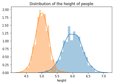
In this case, will we be creating a correct model if we fit one gaussian? No. Here we can see that we need two gaussian to fit the data. Therefore we need two distributions to generalize on the dataset. Therefore, our modeling equation for the mixture of 1-D Gaussians will be:

$$P(x) = \pi_1N(\mu_1, \sigma_1^2) + \pi_2N(\mu_2, \sigma_2^2)$$

where \(\pi_1\) and \(\pi_2\) are the proportion in which the Gaussians are mixed.

Another example is Speech Recognization. "Speech Recognition" case involves 2D data, and we need to fit multiple Gaussians based on the application. We need to update our Gaussian parameters for a 2D Gaussian.

How to model 2-D Gaussian Distribution?

So far we have seen when we have a single variable, how the Gaussian distribution works. We have thereafter also seen the mixture of 1-D gaussian distributions.

Let's move forward and explore when we have two different variables. To represent gaussian in 2D, we use iso-contour, and the alignment and the shape depend upon the covariance matrix.

The contour shape and directions give a lot of information about the data behavior.

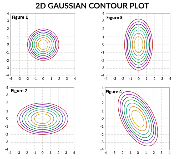
• Figure 1, represents that \(x_1\) and \(x_2\) are not correlated and we will be having all 0's in non-diagonal elements.
• Figure 2, represents that variation along \(x_1\) is more than \(x_2\). Still, variation among \(x_1\) and \(x_2\) is still 0 and we will have 0's in non-diagonal elements.
• Figure 3, represents that variation along \(x_2\) is more than \(x_1\). Still, variation among \(x_1\) and \(x_2\) is still 0 and we will have 0's in non-diagonal elements.
• Figure 4, represents that \(x_1\) and \(x_2\) are negatively correlated. And there will be some correlation between the two. If the shape would have been tilted another way, it would have represented the positive correlation.

I have explained contours in the post, Lasso and Ridge Regression Detailed Explanation. Please refer to it, if you want to revise your concepts.

The equation of 2-D gaussian looks like,

$$P(x) = \sum_{k=1}^k\pi_kN(\mu_k, \sum_k)$$

where \(\sum_k\) is a covariance matrix which along the diagonals represents the variance of individual variables and other elements of the covariance matrix represent the variance of variables between themselves.

Estimating Parameters in GMM Model

After looking at the equation, let's move forward and understand how the estimation in GMM works. We will be doing calculations considering that we are training a GMM model in 2-D space. The same can be generalized in the higher space dimension as well.

K-Means (Unsupervised Learning k-means clustering algorithm in Python) has two steps for making clusters, i.e. Assignment steps and Optimization steps. Similarly, for GMMs, we have the steps called the Expectation step and Maximisation step.

Summarization of the steps that we do in K-means:

• Initialise the cluster centres.
• Perform the Assignment step.
• Optimize the cluster centers.
• Reiterate through steps 2 and 3

Now let's look at the steps that we perform for the Gaussian Mixture Models.

Expectation Step

To initialize the GMMs algorithm we can use K-Means to compute \(\mu_1\) and \(\mu_1\). We can give equal weight to the Gaussians say \(\pi_1\)=0.5 and \(\pi_1\)=0.5, and then we can compute responsibilities that a cluster takes for each data point. Expectation steps assign each data point with a probability known as the soft assignment which is also known as the responsibility that a cluster takes for each data point.

Maximization Step

For K-Means, we recompute the cluster centers as part of the optimization step after we have assigned each data point to a cluster. For GMMs we have a similar step in which we recompute the cluster centers \(\mu_1\) and \(\mu_2\) along with covariance matrix \(\sum\).

For 2-D Gaussan distribution, the parameters that we need to optimize are: \(\pi_1\),  \(\pi_2\),  \(\mu_1\),  \(\mu_2\), \(\sigma^2_1\) and \(\sigma^2_2\).

The responsibility matrix denotes who is taking ownership of the points.

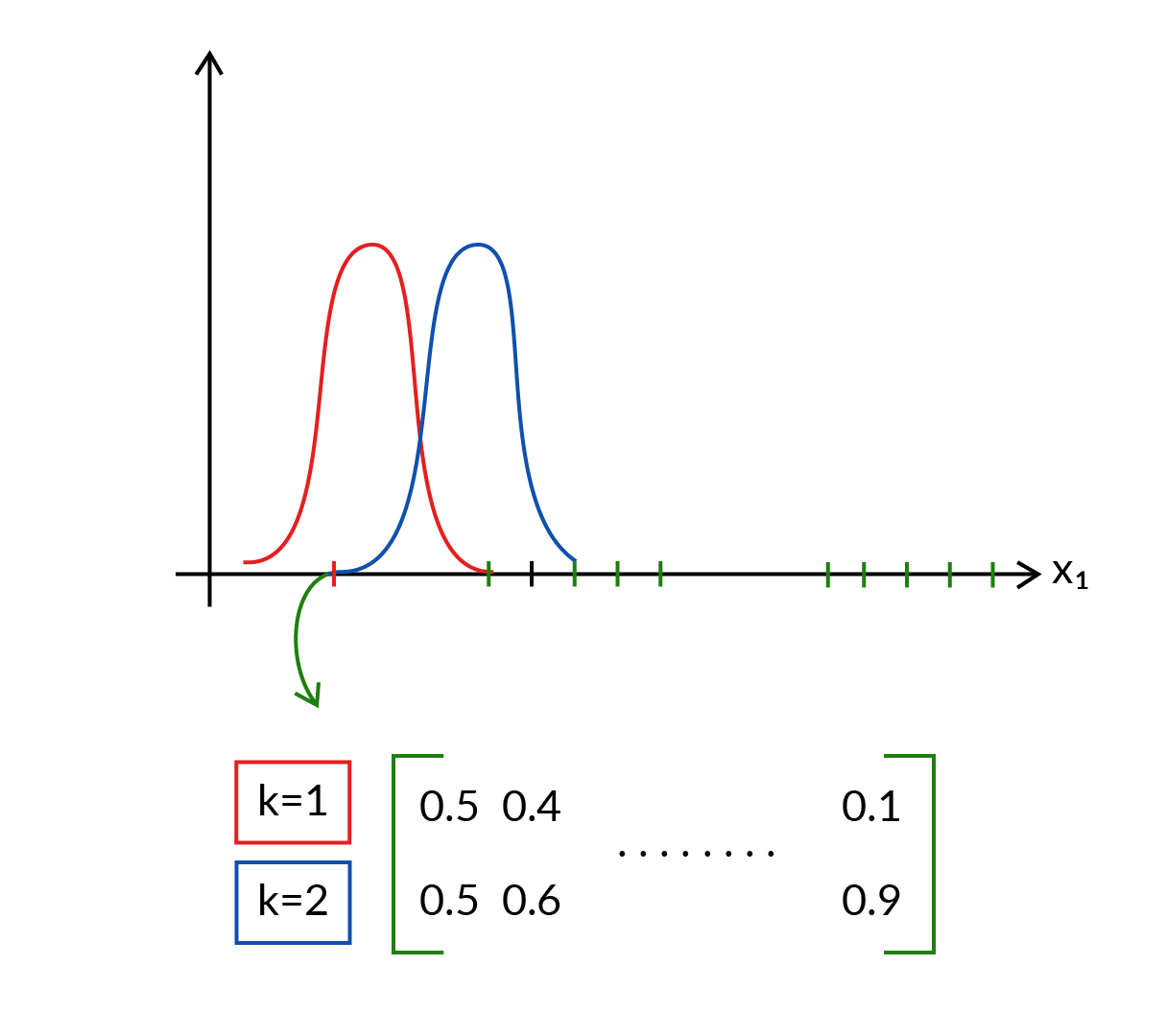
Note: We don't have to compute \(\pi_2\) as it will be 1- \(\pi_1\) as the sum of \(\pi\) should always be 1.

The above diagram shows, clusters 1 and 2 taking equal responsibility for the first data point. But for the second data point, cluster 2 is taking more responsibility as compared to cluster 1. And so on for other data points.

In k-means \(r_{ik}\) is the responsibility matrix, whose responsibility is the cluster to which the data point belongs to the 0 or 1 cluster and in GMM the \(r_{ik}\) states the probability between 0 to 1 for data points belonging to the clusters.

$$\mu_k = {{\sum_{i=1}^N r_{ik}x_i} \over {\sum_{i=1}^Nr_{ik}}}$$

In a similar way, we can find out the \(\sigma^2\) and \(\pi\). The equation derivation is out of scope. Refer to the documentation to know more.

Summary

To summarize, for GMMs, we initialize the parameters(by using K-Means or randomly), and then in the expectation step, we compute the responsibilities for every data point that a cluster takes, and lastly, in the Maximisation step, we recompute the parameters. We keep doing this iteratively until convergence.