Unleashing the Power of Advanced Lexical Processing: Exploring Phonetic Hashing, Minimum Edit Distance, and PMI Score

December 20, 2023

In the post, Demystifying NLP: Exploring Lexical, Syntactic, and Semantic Processing for Powerful Natural Language Understanding under the "Lexical Processing" section we have explored some of the basic techniques including Word Frequencies, Stop words removal, Tokenization, Bag-of-Words Representation, Stemming, Lemmatization, and TF-IDF Representation for lexical processing.
If you are not sure about the above-mentioned techniques or want to revise the topics, I would highly encourage you to go through the above post before moving forward. This post is in continuation to explore advanced techniques that we can use to lexically process the textual data.
In this post, we will be covering some of the advanced techniques used for lexical processing such as Phonetic Hashing, Edit Distance algorithm, and Pointwise Mutual Information. Let's dive straight into it and start understanding phonetic hashing first.
Phonetic Hashing
Canonicalisation refers to the process of reducing any given word to its base word. Stemming and lemmatization are two such techniques to canonicalize words to their base forms. Similarly, Phonetic Hashing is also a popularly used advanced canonicalization technique that can handle the cases that both Stemming and lemmatization fail to handle. Consider an example shown below:
Two misspelled versions of the word ‘disappearing’ - ‘dissappearng’ and ’disappearing’. After we stem these words using Stemming, we still have two different stems - ‘dissappear’ and ‘dissapear’. Lemmatization won't work on these words as it works only on correctly spelled words.
In such cases, we need advanced techniques like Phonetic Hashing to reduce a word to the base form. There are two ways to deal with the above problem:
- Use Soundex algorithm to deal with different spelling because of pronunciation
- Correct the spelling using a technique like minimum edit distance and then apply Stemming or Lemmatization.
Let's first use the Soundex algorithm to solve the problem.
Soundex Algorithm
Certain words have different pronunciations in different languages. As a result, they end up being spelled differently. For example colour and color.
Phonetic hashing buckets all the similar phonemes (words with similar sound or pronunciation) into a single bucket and gives all these variations a single hash code. (i.e. colour and color will have the same code). And it is done using the Soundex algorithm.
Let's understand the step-by-step flow to convert the word using the Soundex algorithm with the help of an example 'Chandigarh'.
- Phonetic hashing is a four-letter code. The first letter of the code is the first letter of the input word. Therefore our first letter of code will be 'C'.
- Next, we need to map all the consonant letters except vowels and 'H', 'Y', and 'W' as {"BFPV": "1", "CGJKQSXZ": "2", "DT": "3", "L": "4", "MN": "5", "R": "6"} We get the code as Cha53i2a6h.
- Next, we keep all the vowels as is in the code, and ‘H’s, ‘Y’s, and ‘W’s are removed from the code. Therefore we get the code as Ca53i2a6.
- The third step is to remove all the vowels. Therefore we get the code as C5326.
- Next, we need to merge all the consecutive duplicate numbers into a single unique number. (All the ‘2’s are merged into a single ‘2’ and so on). We don't have any consecutive duplicates for our example, therefore this step can be skipped.
- The last step is to force the code to make it a four-letter code.
- We either need to pad it with zeroes in case it is less than four characters in length.
- Or truncate it from the right side in case it is more than four characters in length.
- After trimming we get our final code as C532. So the final phonetic hashing of the word 'Chandigarh' is C532.
Below given Python example shows Phonetic hashing algorithm and performing the steps involved as discussed above:
import ast, sys
word = sys.stdin.read()

# define a function that returns Soundex of the words that is passed to it
def get_soundex(token):
    """Get the soundex code for the string"""
    token = token.upper()

    soundex = ""

    # first letter of input is always the first letter of soundex
    soundex += token[0]

    # create a dictionary which maps letters to respective American soundex codes. Vowels
    # and 'H', 'W' and 'Y' will be represented by '.'
    dictionary = {"BFPV": "1", "CGJKQSXZ":"2", "DT":"3", "L":"4", "MN":"5", "R":"6",
                         "AEIOUHWY":"."}

    for char in token[1:]:
        for key in dictionary.keys():
            if char in key:
                code = dictionary[key]
                if code != soundex[-1]:
                    soundex += code

    # remove vowels and 'H', 'W' and 'Y' from soundex
    soundex = soundex.replace(".", "")

    # trim or pad to make soundex a 4-character code
    soundex = soundex[:4].ljust(4, "0")

    return soundex

# store soundex in a variable
# TODO
word = "color" # colour
soundex = get_soundex(word)

# print soundex -- don't change the following piece of code.
print(soundex)
Now, let us take an example of two words ‘color’ and ’colour’ which cannot be resolved using techniques like stemming and lemmatization and applying Phonetic hashing. We see that, for both of the words Phonetic hashing code is the same i.e., C460. Hence we are successfully able to canonicalize using Phonetic hashing which we were not able to do using the stemming and lemmatization algorithm.
Edit Distance
We explored how to deal with different pronunciations, but the Phonetic hashing will not work in case of misspelling. So we need to spell corrector in this case to handle misspellings. We use edit distance which is defined as a distance between two strings that is a non-negative integer number to build a spell corrector algorithm.
One of the algorithms available to calculate the minimum edit distance is the Levenshtein edit distance algorithm. It calculates the number of steps (insertions, deletions, or substitutions) required to go from source string to target string which are defined as follows:
- Insertion of a letter in the source string. For example, to convert 'color' to 'colour', we need to insert the letter 'u' in the source string.
- Deletion of a letter from the source string. For example, to convert 'Matt' to 'Mat', we need to delete one of the 't's from the source string.
- Substitution of a letter in the source string. For example, to convert 'Iran' to 'Iraq', we need to substitute 'n' with 'q'.
Minimum edit distance is an example of dynamic programming. It finds the path that leads to the minimum possible edits.
If we try calculating the edit distance between ‘deleterious’ and ‘deletion’ it is not as straightforward as we have seen for the example above. Hence, we need to understand how to calculate the edit distance between any two given strings, however long and complex they might be.
Let's understand first how the Levenshtein edit distance algorithm works with the help of two words "acquire" and "acquire" where the letter 'c' is missing. We know that there is one insertion needed therefore edit distance of the algorithm will be 1. But this simple example will help us understand how the Levenshtein edit distance algorithm works.
We start by creating the metrics where we align the first word across the row and the second word across the column. We also have a row and column for the null character which is represented as '.' in the example shown below. Therefore, the matrix size that we have is (M + 1) x (N + 1) = 7 x 8.
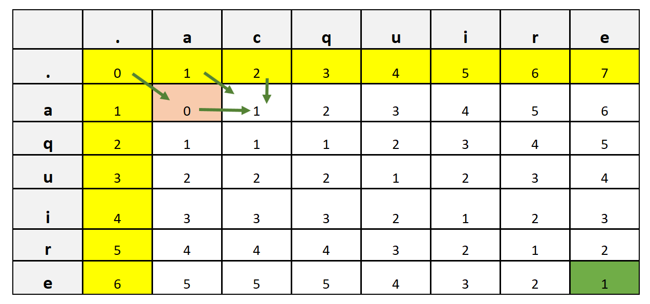
We then start feeling the columns and rows, about how many edits (insertion, deletion, or substitution) we need to move from one letter on a column to another letter on a row. For example, to move from null to null we need 0 edits. To move from null to letter 'a' across a row we need 1 edit and so on. In this way, we fill all the rows and columns highlighted in 'yellow' color above.
Next, to fill in the remaining values, we see if the value of the row and column is the same, then we fill it with the diagonal value. For example, Consider (a, a) where both row and column letter is the same then we have filled with the diagonal value represented by arrow in the image shown above.
If the row and column value is not the same, for example (a, c) then we take a minimum of three preceding neighbors i.e., (i - 1, j), (i, j - 1), and (i - 1, j - 1) and add 1 to it. To fill (a, c) we will take a minimum of (., c), (a, a), and (., a) which is 0 and after adding 1, we get 0 + 1 = 1. We repeat the same step to fill the entire table.
At the end, we get the last column and row value highlighted in green color which represents the total edit distance between two words. Let's attempt to code the same algorithm in Python as shown below:
def lev_distance(source='', target=''):
    """Make a Levenshtein Distances Matrix"""

    # Get length of both strings
    n1, n2 = len(source), len(target)

    # Create matrix using length of both strings - source string sits on columns, target string sits on rows
    matrix = [ [ 0 for i1 in range(n1 + 1) ] for i2 in range(n2 + 1) ]

    # Fill the first row - (0 to n1-1)
    for i1 in range(1, n1 + 1):
        matrix[0][i1] = i1

    # Fill the first column - (0 to n2-1)
    for i2 in range(1, n2 + 1):
        matrix[i2][0] = i2

    # Fill the matrix
    for i2 in range(1, n2 + 1):
        for i1 in range(1, n1 + 1):

            # Check whether letters being compared are same
            if (source[i1-1] == target[i2-1]):
                value = matrix[i2-1][i1-1]                      # top-left cell value
            else:
                value = min(matrix[i2-1][i1]   + 1,             # left cell value     + 1
                            matrix[i2][i1-1]   + 1,             # top cell  value     + 1
                            matrix[i2-1][i1-1] + 1)             # top-left cell value + 1

            matrix[i2][i1] = value

    # Return bottom-right cell value
    return matrix[-1][-1]
Now if we calculate the lev_distance('cat', 'cta') we get output as 2 which makes sense. Also if we see the advance example of ‘deleterious’ and ‘deletion’ we get output as 4.
We can calculate the Levenshtein minimum edit distance using Python simply using the 'edit_distance' method available in the nltk library.
from nltk.metrics.distance import edit_distance

edit_distance('string1', 'string2')
There is another variation of the edit distance i.e., Damerau–Levenshtein distance. The Damerau–Levenshtein distance, apart from allowing the three edit operations, also allows the swap operation between two adjacent characters which costs only one edit instead of two.
We can calculate the Damerau-Levenshtein minimum edit distance using Python as shown below:
from nltk.metrics.distance import edit_distance

edit_distance("apple", "appel", transpositions=False)
The swap operation can be achieved by setting the additional 'transpositions' parameter as false.
Spell Corrector Algorithm
So far we have covered how to find a edit distance between two words. Such a simple algorithm can be used to develop a spell corrector application. The below Python code represents how we can build Norvig’s spell corrector using a minimum edit distance algorithm.
import re
from collections import Counter

def words(document):
	"Convert text to lower case and tokenize the document"
	return re.findall(r'\w+', document.lower())

# Create a frequency table of all the words of the document
# TODO: Need a corpus of corrected spelled words for domain/application
all_words = Counter(words(open('correct_words_corpus.txt').read()))

def edits_one(word):
    "Create all edits that are one edit away from `word`."
    alphabets    = 'abcdefghijklmnopqrstuvwxyz'
    splits     = [(word[:i], word[i:])                   for i in range(len(word) + 1)]
    deletes    = [left + right[1:]                       for left, right in splits if right]
    inserts    = [left + c + right                       for left, right in splits for c in alphabets]
    replaces   = [left + c + right[1:]                   for left, right in splits if right for c in alphabets]
    transposes = [left + right[1] + right[0] + right[2:] for left, right in splits if len(right)>1]
    return set(deletes + inserts + replaces + transposes)

def edits_two(word):
    "Create all edits that are two edits away from `word`."
    return (e2 for e1 in edits_one(word) for e2 in edits_one(e1))

def known(words):
    "The subset of `words` that appear in the `all_words`."
    return set(word for word in words if word in all_words)

def possible_corrections(word):
    "Generate possible spelling corrections for word."
    return (known([word]) or known(edits_one(word)) or known(edits_two(word)) or [word])

def prob(word, N=sum(all_words.values())):
    "Probability of `word`: Number of appearances of 'word' / total number of tokens"
    return all_words[word] / N

def rectify(word):
    "return the most probable spelling correction for `word` out of all the `possible_corrections`"
    correct_word = max(possible_corrections(word), key=prob)
    return correct_word
The above code has a prerequisite to work, where we need to pass correctly spelled known seed documents. A seed document acts like a lookup dictionary for a spelling corrector since it contains the correct spellings of each word.
Now, let’s look at what each function does and understand how the spell corrector algorithm works.
- words(): The function words() is pretty straightforward. It tokenizes any document that’s passed to it.
- Counter: The ‘Counter’ class, creates a frequency distribution of the words present in the seed document. Each word is stored along with its count in a Python dictionary format. We could also use the NLTK’s FreqDist() function to achieve the same results.
- edits_one(): The edits_one() function creates all the possible words that are one edit distance away from the input word. Most of the words that this function creates are garbage, i.e. they are not valid English words.
For example, if we pass the word ‘laern’ (misspelling of the word ‘learn’) to edits_one(), it will create a list where the word ‘lgern’ will be present since it is an edit away from the word ‘laern’. But it’s not an English word. Only a subset of the words will be actual English words.
- edits_two(): Similar to the edit_one() function, the edits_two() function creates a list of all the possible words that are two edits away from the input word. Most of these words will also be garbage.
- known(): The known() function filters out the valid English word from a list of given words. If the words created using edits_one() and edits_two() are not in the dictionary, they’re discarded.
- possible_corrections(): The function possible_corrections() returns a list of all the potential words that can be the correct alternative spelling.
For example, let’s say the user has typed the word ‘wut’ which is wrong. Multiple words could be the correct spelling of this word such as ‘cut’, ‘but’, ‘gut’, etc. This function will return all these words for the given incorrect word ‘wut’. But, how does this function find all these word suggestions exactly? It works as follows:- It first checks if the word is correct or not, i.e. if the word typed by the user is present in the dictionary or not. If the word is present, it returns no spelling suggestions since it is already a correct dictionary word.
- If the user types a word that is not a dictionary word, then it creates a list of all the known words that are one edit distance away. If there are no valid words in the list created by edits_one() only then this function fetches a list of all known words that are two edits away from the input word.
- If there are no known words that are two edits away, then the function returns the original input word. This means that there are no alternatives that the spell corrector could find. Hence, it simply returns the original word.
Some of us might have a question, Why we are passing the seed document? It would have been much better if we could have directly used the dictionary instead of a book. The answer to this question lies in the prob() function of the Python code defined above.
- prob(): The function returns the probability of an input word. This is exactly why you need a seed document instead of a dictionary. A dictionary only contains a list of all correct English words. But, a seed document not only contains all the correct words but it could also be used to create a frequency distribution of all these words. This frequency will be taken into consideration when there is more than one possible correct word for a given misspelled word.
For example, Consider the input word ‘wut’. The correct alternative to this word could be one of these words - ‘cut’, ‘but’ and ‘gut’, etc. The possible_corrections() function will return all these words. But the prob() function will create a probability associated with each of these suggestions and return the one with the highest probability.
I hope the spell corrector algorithm is fun and feel free to play around with this for your applications.
Pointwise Mutual Information
Till now we have explored techniques to achieve canonicalisation. There is still one more bug in the room to address though. Consider following Indian colleges such as ‘The Indian Institute of Technology, Bangalore’, ‘The Indian Institute of Technology, Mumbai’, ‘The National Institute of Technology, Kurukshetra’ and many others colleges.
Now, when we tokenize this document, all these college names will be broken into individual words such as ‘Indian’, ‘Institute’, ‘International’, ‘National’, ‘Technology’, and so on which is not correct and we want an entire college name to be represented by one token.
How do we tackle this problem of tokenization? Any thoughts?
As the topic suggests, there is a metric called pointwise mutual information, also called the PMI. We can calculate the PMI score of each of these terms. PMI score of terms such as ‘Indian Institute of Technology, Bangalore’ will be much higher than other terms. If the PMI score is more than a certain threshold then you can choose to replace these terms with a single term such as ‘Indian_Institute_of_technology_Bangalore’.
The same is the case with other words such as Hong Kong. Let's understand how we can calculate the PMI score.
Calculating PMI score
Here we calculate the PMI score of every word in the corpus. And words like Hong Kong will have a high PMI score. So, If the PMI score is more than a certain threshold then we can choose to replace these terms with a single term such as ‘Hong_kong’.
The formula to calculate the PMI score for Hong Kong or two-letter words is given:
$$P(x,y) = log({P(x,y) \over P(x) P(y)})$$
where x and y represent the words. And, p(x,y) is the joint probability whereas p(x) and p(y) are the marginal probabilities of the words ‘x’ and ‘y’. To compute the probabilities as stated in the PMI formula, we need to decide on the occurrence context. Like:
- Words as the occurrence context: P(w) = Number of times given word ‘w’ appears in the text corpus/ Total number of words in the corpus
- The sentence as the occurrence context: P(w) = Number of sentences that contain ‘w’ / Total number of sentences in the corpus
- Paragraph as the occurrence context: P(w) = Number of paragraphs that contain ‘w’ / Total number of paragraphs in the corpus
Based on the occurrence context we can calculate the PMI score of the given words. Let's take an example of the following three sentences as a corpus and calculate the PMI score of the word "New Delhi" considering each sentence as an occurrence context.
- S1: Construction of a new metro station state in New Delhi
- S2: New Delhi is the capital of India
- S3: The climate of Delhi is a monsoon-influenced humid climate
We can calculate the probabilities P(New Delhi) = 2/3, P(New) = 2/3, P(Delhi) = 3/3. Next, we can easily calculate the PMI score of the term "New Delhi" as, PMI(New Delhi) = p(New Delhi) / (p(New) x P(Delhi). This is how PMI score calculation works.
After calculating the PMI score, we can compare it with a cutoff value and see if the PMI is larger or smaller than the cutoff value. A good cutoff value is zero.
Terms with PMI larger than zero are valid terms, i.e. they don’t need to be tokenized into different words. Therefore, we can replace these terms with a single-word term that has an underscore present between different words of the term. For example, the term ‘New Delhi’ has a PMI greater than zero. It can be replaced with ‘New_Delhi’. This way, it won’t be tokenized while using the NLTK tokenizer.
N-Gram Models
Calculating the PMI score for a two-word term was pretty straightforward. But when you try to calculate the PMI of a three-word term such as 'Indian Institute of Technology'. In this case, we will have to calculate P(Indian Institute Technology). To calculate such probability, we need to apply the chain rule of probability.
Using the chaining rule we can calculate the PMI for the longer phrases as shown below:
$$P(x,y,z) = log ({P(x,y,z) \over P(x) P(y) P(z)})$$
$$P(x,y,z) = log [{(P(z|y, x)*P(y|x))*P(x)\over (P(z)P(y)P(x))}]$$
$$=log [{(P(z|y, x)*P(y|x)) \over ([P(z)P(y))}]$$
Similarly, we can generalize the equation to calculate the PMI score to n terms. But the chaining rule is very costly to compute, therefore some kind of approximations are used over the chaining rule. A very commonly used approximation is the N-gram model.
The N-Gram model is a sequence of 'n' consecutive words from an input stream. Let us understand this with the help of an example: "To be or not to be". Let us calculate the Bigram (which is nothing with n value as 2) of the string. The bigram of the string will be ("To be", "be or", "or not", "not to", "to be")
Now if we want to write a chain rule of the string it will be:
P("To be or not to be") = P(to) P(be|to)P(or|"to be")P(not |"to be or")P(to|"to be or not")P(be|"to be or not to")
But with Bigram approximation our calculation reduces to:
P("To be or not to be") = P(to) P(be|to)P(or|be)P(not|or)P(to|not)P(be|to)
In bigram, we are computing the probability of the term given the previous term instead of computing all the previous terms as we are doing in the chain rule. Using this we can majorly reduce the complexity. Now we can easily count the occurrences of the bigrams and calculate the PMI values.
In practical settings, calculating PMI for terms with more than two is still very costly for any relatively large corpus of text. In such a scenario, we can either go for calculating it only for a two-word term or choose to skip it if we know that there are only a few occurrences of such terms.
Author Info