Mastering Named Entity Recognition: Unveiling Techniques for Accurate Entity Extraction in NLP

In the expansive realm of Natural Language Processing (NLP), Information Extraction (IE)  is a sophisticated technique that processes vast amounts of textual data to pinpoint and extract specific information, transforming the narrative into a structured format that machines can comprehend. It can help in identifying entities, relationships, or events helping machines to distill meaningful knowledge from the linguistic richness of human expression.

In this post, we will build an information extraction (IE) system that can extract entities relevant to booking flights (such as source and destination cities, time, date, budget constraints, etc.) in a structured format from unstructured user-generated queries. We will explore different algorithms available to perform the IE task. IE is used in many applications such as conversational chatbots, extracting information from encyclopedias (such as Wikipedia), etc. A generic IE pipeline is as follows:

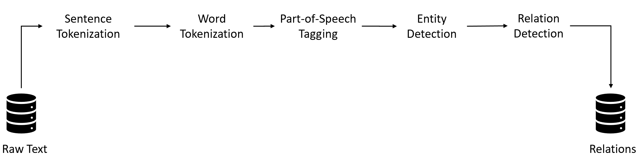
We start with the preprocessing techniques and perform Sentence Segmentation, Word Tokenization, and Part of Speech Tagging. These techniques are covered extensively in the post, Demystifying NLP: Exploring Lexical, Syntactic, and Semantic Processing for Powerful Natural Language Understanding (Lexical Processing section). I will recommend covering the pre-processing techniques first before moving forward.

After performing preprocessing next step is to POS tag the words in a given sentence. Let's explore this next.

POS Tagging

Once the preprocessing of the next is done, we next perform the POS tagging task. POS Tagging approaches using NLTK library in covered in the post, Demystifying Part-of-Speech (POS) Tagging Techniques for Accurate Language Analysis.

However, one important point to note is that NLTK POS tagger is not accurate such as any word after ‘to’ gets tagged as a verb and this will impact our NER model that we want to build for booking flights. For example, in all the queries of the form ‘.. from city_1 to city_2’, city_2 is getting tagged as a verb. This is happening because, The NLTK tagger is trained on a certain training corpus, which probably contains many words in the sequence ‘to/TO word/VB’. In other words, the model’s transition probabilities are providing an incorrect signal.

To correct the POS tags manually, we can use the backoff option in the nltk.tag() method.  The backoff option allows to chain of multiple taggers together. If one tagger doesn’t know how to tag a word, it can back off to another one.

It is difficult to get 100% accuracy in POS tagging which is okay for the NER task as POS tags are just one of the features for prediction, we use other features as well (such as the morphology of words, the words themselves, other derived features, etc.).

Let's start our discussion with the next step i.e., entity detection.

Entity Detection: IOB Labeling

Once we have preprocessed and POS-tagged data, we get to the core task of entity detection. Entity Detection or IOB labeling (also called BIO in some texts) is a standard way of labeling named entities. The IOB method tags each token in the sentence with one of the three labels: I - inside (the entity), O- outside (the entity), and B - beginning (of an entity). Let us consider an example.

Consider the following example for IOB labeling:

If we look at the example above, the word 'Smoke' is beginning, the words 'House' and 'Deli' are inside, and the word 'for' is outside. This task is done as we want our system to read 'Smoke House Deli' as a single entity. Training a NER system, i.e. assigning an IOB label to each word, is a sequence labeling task similar to POS tagging.

But why do we need IOB labeling?

The Named Entity Recognition task identifies ‘entities’ in the text. Entities could refer to names of people, organizations (e.g. Air India, United Airlines), places/cities (Mumbai, Chicago), dates and time points (May, Wednesday, morning flight), numbers of specific types (e.g. money - 5000 INR), etc. POS tagging in itself won’t be able to identify such word entities. Therefore, IOB labeling is required. So, the NER task is to predict the IOB labels of each word.

Once the entities are detected, the final part is to detect and extract the relationships. Let's explore this next.

Relationship Extraction

Let's assume we can achieve the task of sequence labeling (We will be covering algorithms used to achieve this task in the next section of this post), the next step is to combine the labeled tokens based on their labels. Once the words are labeled, the next task is to find the relationship between the entities. There are two popular techniques to achieve this.

Relation Recognition is the task of identifying relationships between the named entities. Using entity recognition, we can identify places (pl), organizations (o), and persons (p). Relation recognition will find the relation between (pl,o), such that o is located in pl. Or between (o,p), such that p is working in o, etc.

Record Linkage refers to the task of linking two or more records that belong to the same entity. For example, Bangalore and Bengaluru refer to the same entity.

With this, our entire IE pipeline is completed.

Algorithms for Entity Detection

Coming back to entity detection which is the core of the IE pipeline, let us understand the different algorithms available to perform the task of entity detection/recognition or sequence labeling.

As for the POS tagging task, there are multiple approaches, the same is the case with IOB labeling or sequence labeling tasks. We can try rule-based models such as writing regular expression-based rules to extract entities, chunking patterns of POS tags into an 'entity chunk' etc. Or, we can use probabilistic sequence labeling models such as HMMs, the Naive Bayes classifier (classifying each word into one label class), Conditional Random Fields (CRFs), etc.

Let's start with the rule-based models. I am also attaching the Jupyter Notebook for you to follow along with the post and run the code side by side.

Rule-Based Models for Entity Recognition

Rule-based taggers use the commonly observed rules in the text to identify the tag of each word. They are similar to the rule-based POS taggers which use rules such as these - VBG mostly ends with ‘-ing’, VBD is likely to end with ‘ed’ etc. Rule-based models for NER tasks are based on the technique called chunking.  Let's explore it next.

Chunking

Chunking is the rule-based approach for Entity Recognization. In chunking, the first step is to identify the POS tag for every word in the sentence. Let's consider an example sentence "We saw the yellow dog".

After POS tagging the sentence we will get an output as We/PRP saw/VBD the/DT yellow/JJ dog/NN. The next step is where we define the grammar to identify noun phrase chunks in the sentence. For example, we define grammar as given below:

Grammar: 'NP_chunk: {<DT>?<NN>}'

After applying grammar "the yellow dog" will be identified as the chunk. Using chunking we can easily do IOB tagging as given below:

We/B-NP saw/O the/B-NP yellow/I-NP dog/I-NP. 

Rule-based systems become more complex and difficult to maintain as we keep on increasing the rules. The alternative is to use probabilistic machine learning models. Let's explore this next.

Probabilistic Models

Probabilistic models give the most probable IOB tags for words. There are multiple probabilistic modeling techniques available for the task of entity detection. Let's start with the unigram and bigram models.

Unigram and Bigram Models

The unigram chunker computes the unigram probabilities P(IOB label | pos) for each word and assigns the label that is most likely for the POS tag. And, Bigram chunker works similarly to a Unigram chunker, the only difference being that now the probability of a POS tag having an IOB label is computed using the current and the previous POS tags, i.e. P(label | pos, prev_pos).

Let us understand Python code to train a unigram model for the entity detection task.

# unigram chunker

from nltk import ChunkParserI

class UnigramChunker(ChunkParserI):    
    def __init__(self, train_sents):
        # convert train sents from tree format to tags
        train_data = [[(t, c) for w, t, c in nltk.chunk.tree2conlltags(sent)] 
                      for sent in train_sents]
        self.tagger = nltk.UnigramTagger(train_data)
        
    def parse(self, sentence):
        pos_tags = [pos for (word, pos) in sentence]
        tagged_pos_tags = self.tagger.tag(pos_tags)
        chunktags = [chunktag for (pos, chunktag) in tagged_pos_tags]
        
        # convert to tree again
        conlltags = [(word, pos, chunktag) for ((word, pos), chunktag) in zip(sentence, chunktags)]
        return nltk.chunk.conlltags2tree(conlltags)

unigram_chunker = UnigramChunker(train_trees)

In the same way, we can train a bigram model by using self.tagger = nltk.BigramTagger(train_data) instead of self.tagger = nltk.UnigramTagger(train_data) in the above code.

In the above code, train_trees is assumed to be the POS tag tree structure. Refer to Jupyter Notebook to know details on how the data processing is performed.

Consider a scenario where we have Unigram and Bigram models for POS tagging tasks. Unigram performed much better than the Bigram model (where Unigram had about 85% accuracy, while Bigram had about 15% accuracy). On the other hand, in IOB tagging, the Bigram chunker performs better than Unigram. What do you think is the reason for this?

POS tagging performed better with unigram because most English words like nouns don't depend on previous words and always have the same tag. But in the case of IOB tagging, only the O tag will be assigned properly in the case of Unigram.

Gazetteer: Look Up Dictionary

One more way to identify named entities is to look up a dictionary or a gazetteer. A gazetteer is a geographical directory that stores data regarding the names of geographical entities (cities, states, countries) and some other features related to the geographies. We can generate a dictionary of all possible entities that we have in the corpus. This will have a great impact on improving accuracy.

We can look for the dictionary related to the domain online or use domain experts to create a dictionary that can help significantly improve the accuracy of NER algorithms.

Naive Bayes Classifier for NER

We can also build a machine-learning model to predict the IOB tags of the words. Features could be the morphology (or shape) of the word such as whether the word is upper/lowercase, POS tags of the words in the neighborhood, whether the word is present in the lookup dictionary, etc.

Sequence prediction tasks such as NER can be modeled by classifiers such as Naive Bayes, Decision Trees, etc. The classifier task is where we are given a list of words whose IOB tags are to be predicted. The target label sequence is a vector of IOB labels.

To build classifiers, we create features for each word in the sequence like the word itself, the previous word, the next word, the POS tag, the previous POS tag, the next POS tag, the previous IOB label, word_is_city, etc.

Let's look at Python code that can help train a Naive Bayes classifier for the NER task.

# Extracts features for the word at index i in a sentence 
def npchunk_features(sentence, i, history):
    word, pos = sentence[i]
    
    # the first word has both previous word and previous tag undefined
    if i == 0:
        prevword, prevpos = "<START>", "<START>"
    else:
        prevword, prevpos = sentence[i-1]

    # gazetteer lookup features (see section below)
    gazetteer = gazetteer_lookup(word)

    return {"pos": pos, "prevpos": prevpos, 'word':word,
           'word_is_city': gazetteer[0],
           'word_is_state': gazetteer[1],
           'word_is_county': gazetteer[2]}

class ConsecutiveNPChunkTagger(nltk.TaggerI): 

    def __init__(self, train_sents):
        train_set = []
        for tagged_sent in train_sents:
            untagged_sent = nltk.tag.untag(tagged_sent)
            history = []
            # compute features for each word
            for i, (word, tag) in enumerate(tagged_sent):
                featureset = npchunk_features(untagged_sent, i, history) 
                train_set.append( (featureset, tag) )
                history.append(tag)
        self.classifier = nltk.NaiveBayesClassifier.train(train_set)

    def tag(self, sentence):
        history = []
        for i, word in enumerate(sentence):
            featureset = npchunk_features(sentence, i, history)
            tag = self.classifier.classify(featureset)
            history.append(tag)
        return zip(sentence, history)

class ConsecutiveNPChunker(nltk.ChunkParserI): 
    def __init__(self, train_sents):
        tagged_sents = [[((w,t),c) for (w,t,c) in
                         nltk.chunk.tree2conlltags(sent)]
                        for sent in train_sents]
        self.tagger = ConsecutiveNPChunkTagger(tagged_sents)

    def parse(self, sentence):
        tagged_sents = self.tagger.tag(sentence)
        conlltags = [(w,t,c) for ((w,t),c) in tagged_sents]
        return nltk.chunk.conlltags2tree(conlltags)

chunker = ConsecutiveNPChunker(train_trees)

Similarly, we can train any of the Machine Learning models like Decision Trees, SVM, etc.

Hidden Markov Models for IOB Labeling

We have explored HMMs in detail for building POS taggers in post, Demystifying Part-of-Speech (POS) Tagging Techniques for Accurate Language Analysis. In general, Hidden Markov Models (HMMs) can be used for any sequence classification task, such as NER.

However, because of some limitations of HMMs, they are not preferred for the NER task we are trying to solve. In HMM, we can only use the current word for the task of IOB labeling, but we have seen earlier that in the Naive Bayes Classifier section, we need previous and next words as well for the task of IOB labeling. Therefore, it is difficult to input other features in HMM models.

Apart from this, another challenge with learners is that they learn joint distribution for the sequence of input words and output tags and because of this we require a huge amount of data to learn large HMMs. Therefore, more sophisticated sequence models have been developed and widely accepted in the NLP community. In the rest of the post, we will see how one such CRF algorithm helps solve the problem.

Conditional Random Fields

CRFs are used in a wide variety of sequence labeling tasks such as POS tagging, speech recognition, NER, and even in computational biology for modeling genetic patterns, etc. These are commonly used as an alternative to HMMs, and, in some applications, have empirically proven to be significantly better than HMMs. 

There are two types of classifiers in ML:

1. Discriminative classifiers learn the boundary between classes by modeling the conditional probability distribution P(y|x), where y is the vector of class labels and x represents the input features. Examples are Logistic Regression, SVMs, etc.

2. Generative classifiers model the joint probability distribution P(x,y). The focus is on how features and target variables occur together. The goal is to be able to explain how the data is generated. Once the model captures the process that generated the data, it can make predictions on the new examples (i.e. data points). Examples of generative classifiers are Naive Bayes, HMMs, etc.

CRFs are discriminative probabilistic classifiers (often represented as undirected graphical models in some texts). It models the conditional probability P(Y|X), where Y is the vector of the output sequence (IOB labels here) and X is the input sequence (words to be tagged). In other terms, the task is to predict the IOB label for a given word.

In the CRF algorithm, rather than feeding the input sequence X as it is to the algorithm, we usually derive features from the input sequence and feed the features to CRF models. Next, let us understand what kind of features CRFs generally use.

CRF Feature Functions

The idea behind creating features for CRF is similar to how we extracted features for building the naive Bayes classifiers for the NER task in a previous section. Some examples of word features (these are the features where each word has these features) include word and POS tag-based features such as word_is_city, word_is_digit, pos, previous_pos, etc., or label-based features such as previous IOB label.

NOTE: We restrict the model to extract label-based word features using only the previous label (and not using labels of the previous n words where n > 1). This assumption is similar to the first-order Markov assumption we had used in POS tagging (i.e. transition probabilities depend only on the previous POS tag).

Let’s spend some time to understand CRF features in detail. Consider a sequence of n tokens (or words) \(x=(x_1,x_2,x_3,...x_n)\) and the corresponding IOB label sequence \(y=(y_1,y_2,y_3,...y_n)\). We define some feature functions in CRFs which we’ll denote as f. The defined feature function takes the following four inputs:

1. The input sequence of words: x
2. The position \(i\) of a word in the sentence (whose features are to be extracted)
3. The label \(y_i\) of the current word (the target label)
4. The label \(y_{i-1}\) of the previous word

There are usually multiple feature functions, let’s denote the \(j^{th}\) feature function as \(f_j(x, i, y_i, y_{i−1})\). The feature functions return a real-valued number, which is often 0 or 1 (i.e. binary output).

NOTE: The label information is encoded in the feature itself.

Let’s take an example of a feature function \(f_1\) which returns 1 if the word \(y_i\) is a city and the corresponding label \(y_i\) is ‘I-location’, 0. This can be represented as:

$$f_1(x,i,y_i,y_{i−1})=[[x_i \ is \ in \ city \ list \ name] \ and \ [y_i \ is \ I-location]]$$

The feature function returns 1 only if both conditions are satisfied, i.e. when the word is a city name and is IOB tagged as ‘I-location’ (e.g. Chicago/I-location).

Similarly, a second feature function can be defined using the previous label, for example:

$$f_2(x,i,y_i,y_{i−1})=[[y_{i-1} \ is \ B-location] \ and \ [y_i \ is \ I-location]]$$

We can define multiple such feature functions \(f_i\), though all are not equally important. Every feature function \(f_i\) has a weight \(w_i\) associated with it, which represents the ‘importance’ of that feature function which is almost the same as logistic regression where coefficients of features represent their importance.

State and Transition features

There are two types of feature functions, which are state features and transition features. The state feature is the feature that is defined for the \(i^{th}\) position of the word in a sentence as shown below:

$$f_1(x,i,y_i,y_{i−1})=[[x_i \ is \ in \ city \ list \ name] \ and \ [y_i \ is \ I-location]]$$

The example shown above is creating a dictionary-based state feature. Whereas the transition feature function is defined as dependent on the IOB label of the previous position as shown below,

$$f_org(x,i,y_i,y_{i−1})=[[x_i \ is \ in \ org \ dict] \ and \ [y_i \ is \ I-org] \ and \ [y_{i - 1} \ is \ B-org]]$$

Therefore, labeling the previous word in a sequence is important for defining transition probability.

To summarize there are different types of features that we can define for the CRF model such as dictionary features, word features, POS features, and orthographic features.

HMMs also have two kinds of probabilities associated with them which are Transition and Emission Probability. Transition probability is similar to transition features and Emission probability is similar to the state features is the analogy between HMMs and CRFs.

Once we have computed the features for the CRF model, the next step is to train a CRF model where the goal is to learn the importance of different feature functions. Let's explore what we mean by training the CRF model.

Training a CRF

Training a CRF means to compute the optimal weight vector w which best represents the observed sequences y for the given word sequences x. In other words, we want to find the set of weights w which maximizes P(y|x,w). This is similar to training a logistic regression model to find the optimal coefficients by maximizing P(y|x,w) where w represents the vector of logistic regression model coefficients.

Before going and learning about CRF model training, let’s first focus on the model architecture. Similar to logistic regression where the conditional probability P(y|x,w) is modeled using a sigmoid function. You can refer to the post, Logistic Regression Detailed Explanation. In CRFs, we model the conditional probabilities P(y|x,w) in a very similar way. There are k feature functions (and thus k weights), for each word 'i' in the sequence x, we define a scoring function as follows:

$$score_i=exp(w_1.f_1+w_2.f_2…+w_k.f_k)=exp(w.f(y_i,x_i,y_{i−1},i))$$

The intuition for the score of the \(i^{th}\) word is that it returns a high value if the correct tag is tagged to the word, else a low value.

Let us understand this with the help of example, say we want to tag the word ‘Francisco’ in the sentence ‘The flight to San Francisco.’ Consider that we have only two feature functions \(f_1\) and \(f_2\) defined the same as we have seen earlier in the CRF feature function section. Now, if we assign the (correct) label ‘I-location’ to ‘Francisco’, both \(f_1\)  and \(f_2\) return a 1, and they return a 0 for any other tag such as ‘O’. Also, exp(x) being a monotonically increasing function, it returns a high value for high values of x. Thus, the score of a word is high when the correct tag is assigned to a word.

The score above is defined for each word in the sequence x. If the sequences x and y are of length n, then the score of the sequence y is given by the product of scores of individual words in x. The sequence score will be highest when all the words have been assigned the correct labels:

$$sequence \ score(y|x) = ∏^n_{i=1}(exp(w.f(y_i,x_i,y_{i−1},i)))$$

The product of exponents can be expressed as the exponential of the sums as follows:

$$sequence \ score(y|x) = ∏^n_{i=1}(exp(w.f(y_i,x_i,y_{i−1},i))) =exp(∑^n_1(w.f(y_i,x_i,y_{i−1},i)))$$

Scores to Probabilities

Using some math, we can now translate the scores of label sequences as defined above, which can be any real numbers to probabilities. The probability P(y|x,w), i.e. the probability of observing the sequence y  given x for a certain weight of feature functions w, is given by the score of the sequence y divided by the total score of all possible label sequences. If we have n words and t IOB labels, there are \(t^n\) possible IOB sequences y. The inference task is to find the optimal sequence y.

The probability of observing the label sequence y given the input sequence x is given by:

$$P(y|x, w) = exp(∑^n_1(w.f(y_i,x_i,y_{i−1},i)))/ Z(x) = exp(w.f(x,y))/Z(x)$$

= score of sequence y assigned to x / sum of scores of all possible sequences

The denominator in the following expression, Z(x), if there are N possible sequences \((N=t^n)\), is a normalizing constant that represents the sum of scores of all possible label sequences of x given by:

$$Z(x)=∑^N_1(exp(w.f(x,y))$$

Defining training objective function

After converting the score to probabilities, let us move forward and consider N such sequences (i.e. N sentences along with their IOB labels), assuming that the sequences are independent, we want to maximize the product of likelihoods of all sequences, i.e. \(∏^N_1(P(y|x,w))\).

Now, if we have N such (x,y) sequences, the training task is to find weights w which maximizes the probability of observing the N sequences (x,y). The objective is to find the weight vector w such that P(y|x,w) is maximized. If there are N sequences, assuming that the N sequences are independent of each other, the likelihood function to be maximized is:

$$L(w|x,y)=P(Y|X,w)=∏^N_1(P(y|x))$$

Since the likelihood function is exponential, we take a log on both sides to simplify the computation (this makes sense since log(x) is a monotonically increasing function, and thus, maximizing x is equivalent to maximizing log(x)):

$$L(w|x,y)=log(P(Y|X,w))=∑^N_1(log(P(y|x,w))$$

From our earlier equation defined above for P(y|x,w) and substituting this in the equation we get:

$$L(w|x,y)=∑^N_1(log(exp(w.f(x,y)/Z(x)))=∑^N_1(log(exp(w.f(x,y))−log(Z(x)))=∑^N_1(w.f(x,y)−log(Z(x)))$$

To prevent overfitting, we use the regularization term:

L(w)=∑[(w.f)−log(Z)] - regularisation_term

Thus, we now have the objective function to be maximized.

Next, let's explore how we can maximize the log-likelihood equation using gradient descent. I suggest refreshing the concept of gradient descent before moving forward. Refer to the post, Simple Linear Regression detailed Explanation.

The final equation after taking the gradient of the log-likelihood function is:

$$ L(w)=∑^N_1(f(x,y))−E_{p_v(y|x,w)}(f(x,y′))−2w/C$$

where,

$$E_{p_v(y|x,w)}(f(x,y′))=∑N1f(x,y′)∗exp(w.f(x,y′))/z_w(x)$$

So, we start with a random initial value of the weights w, and in each iteration, we adjust w to move in the direction of increasing cost. This direction is given by the gradient of the log-likelihood function.

Once we have maximized the likelihood function to find the optimal set of weights, we can use them to infer the labels for a given word sequence. With this, we complete the definition of the objective function for the IOB labeling task using the CRF model. 

Predicting using CRF models

To get the most probable label sequence, \(t^n\) calculations need to be performed which is very similar to HMM models. Therefore, we will be taking motivation from HMM to predict IOB labels using CRF models.

The inference task to assign the label sequence \(y^*\) to x which maximizes the score of the sequence, i.e.

$$y^∗=argmax(w.f(x,y))$$

The naive way to get \(y^*\) is by calculating w.f(x,y) for every possible label sequence y, and then choosing the label sequence that has maximum (w.f(x,y)) value. However, there are an exponential number of possible labels (\(t^n\) for a tag set of size t and a sentence of length n), and this task is computationally heavy.

The difference between HMM and CRF is that HMM puts a constraint on the current label to be dependent only on the current word and previous label. While CRFs can use more features like all the words in a sentence, etc.

Let us take an example and define three feature functions with weights as follows. Also, for simplicity, assume that the task is to only find cities and there are only possible labels ‘O’ for outside an entity and ‘C’ for city:

• \(w_{trans}=3; F_{trans}:y_{i−1}=O , x_i \ is \ in \ city_{dict} , \)

• \( w_{trans}=2; \& \ y_i=O \)

• \( w_{dict}=5; f_{dict}=x_i \ is \ in \ city_{dict} \ \& \ y_i=C \)

The first feature will return 1 if the label is C, the previous label is O (i.e. it transitions from O to C), and if the word is in the city dictionary. Since the weight of the first feature function is 3, it returns 3 if these conditions are satisfied. Similarly, we can interpret the other feature functions. The second function returns 2 if two ‘O’s appear consecutively, while the third function returns 5 if the word is in the city dictionary.

Using the above-mentioned feature function, let's now try to make an inference for the sentence: "Fly to Atlanta".

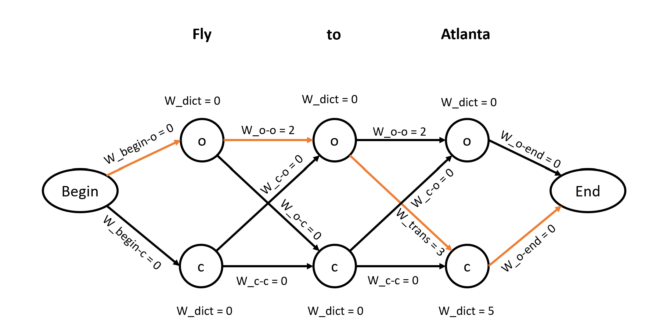
The diagram above shows that there are two possible labels for each word. And since we have a chain CRF the graph is defined as shown above. Here, we will go through every node and every path between the nodes and assign the weights on edges and nodes using the feature function definition.

Next, the goal is to find the path that has the maximum weight on it. To find the path with maximum weight we will be adding up the weight of nodes and path. To solve the problem of finding the maximum weight path we can find such a path in a brute force way but it will be computationally expensive. Therefore, we use dynamic programming here to find the path with maximum weight.

Let's say we were able to find the path using dynamic programming as highlighted in orange color in the image shown above. Therefore the IOB label for the words "Fly to Atlanta" will be o-o-c. In this way, we perform the prediction task once we know the weights of the feature functions from training.

CRF algorithm can be coded using the sklearn_crfsuite package as shown below:

import sklearn_crfsuite

crf = sklearn_crfsuite.CRF(
    algorithm='lbfgs',
    c1=0.01,
    c2=0.1,
    max_iterations=100,
    all_possible_transitions=True
)
crf.fit(X_train, y_train)

To know more details on how we can use the CRF algorithm for NER tasks refer to the Jupyter Notebook.