Hypothesis Testing explained using practical example

There are a lot of articles/blogs that you can find on hypothesis testing. But I still feel the need to write one because when I understood Hypothesis Testing, I failed to find one that can intuitively tell real-world examples of how we can use Hypothesis Testing. Inspired by the book "Naked Statistics - Stripping the dread from the Data" by Charles Wheelan, this is my attempt to explain hypothesis testing.

A hypothesis test evaluates two mutually exclusive statements about a population to determine which statement is best supported by the sample data.

Let's look at the process of performing hypothesis testing:

1. State null hypothesis - We state the statement assuming (prevailing belief about the population) that the value that we are trying to calculate is true/false.
2. Define test statistics - We define statistics in which we are interested in calculating. E.g., mean, median, std, etc.
3. Generate many sets of simulated data assuming the null hypothesis is true - We follow permutation to generate sets.
4. Compute test statistics for each generated simulated dataset - We compute the test statistics for every simulated dataset.
5. Calculate p-value - Once we are done with the calculations, we compute the p-value. If the p-value is equal to or above the significance level, we accept the null hypothesis; otherwise, we reject it.

Now let's get into details and try to understand the concept intuitively.

Any statistical inference begins with an implicitly or explicitly defining null hypothesis. Defining the null hypothesis is our starting assumption, which will be rejected based on the statistical analysis. We will discuss this further in this post.

• If we reject the null hypothesis, we typically accept some alternative hypothesis that we have defined as more consistent with the observed data.
   
• It may also happen that we fail to reject the null hypothesis. If one study has failed to reject the null hypothesis doesn't mean that it's a universal fact as the test is performed on the sample and not the entire population. Because of this reason, we never accept the null hypotheses.

Example: Let us take the example of the court to understand. In court, the law states that the defendant is innocent (null hypothesis). The prosecution's job is to reject the assumption and accept the alternative hypothesis (the defendant is guilty). If the defendant is found guilty, it means the judge rejects the null hypothesis. The judge decides that there is enough evidence to support the alternative hypothesis.

Alternatively, the judge acquits the defendant, which means there is no evidence to support the alternative hypothesis. Note that it doesn't mean the defendant is innocent; it only means there is not enough evidence.

NOTE: We cannot accept null hypothesis, we can only fail to reject it.

I hope the reason is quite clear.

It may seem counterintuitive, but research often creates null hypotheses in the hope of rejecting them. But how implausible does the null hypothesis have to be before we can reject it and accept some alternative explanation? Or, in our example, how can a judge define "enough evidence," we need to quantify it.

Significance Level

The answer to the above question is in the significance level, which is decided before starting the experiment. One of the most common thresholds or significance levels used for rejecting the null hypothesis is 5 percent, also written as 0.05.

The significance level represents the upper bound for the likelihood of observing some data pattern if the null hypothesis were true. Let's understand this statement intuitively.

Let's define a significance level of 0.05 or 5 percent. We can reject the null hypothesis at a 0.05 significance level if there is less than a 5 percent chance of getting an outcome at least as extreme as what we have observed if the null hypothesis were true.

Consider an example of a bus having roughly 60 passengers that got missing from an athlete competition. You found a bus and suspect that this is the same missing bus from the athlete competition. Now we have an understanding of what the null and the alternative hypotheses are. Let's define it next for the example:

Null Hypothesis (H0): The bus contains 60 passengers from athlete competition.

Alternative Hypothesis (H1): The Bus doesn't contain 60 passengers who are from athlete competition.

Let us also acquire the domain knowledge that will help us to navigate through the example.

Assumptions/Domain knowledge: You know that the bus has passengers from the athlete competition and can use weight to find it out. Also, assume you magically got to know the weight of individuals on the bus.

• You have calculated the mean weight from individual passenger weights as 136 pounds.
• You also know the mean weight (162 pounds) and standard deviation (36 pounds) of the sample drawn from the athlete competition.
• Also, assume that the sample collected is normally distributed.

Now with this data, we can calculate the standard error (which is the approximate standard deviation of a statistical sample population.) as  \(s / \sqrt n\), which is equal to \(36 / \sqrt 60\) = 4.6. As the Central Limit Theorem states, if the data is distributed around the mean following the bell shape curve, then

• 68% of data lies within one standard error
• 95% of data lies within two standard error
• 99.7% of data lies within three standard error

Therefore we will expect 95 percent of 60 passengers to have a mean weight with two standard errors i.e. 153 pounds \((162 - (4.6 * 2))\) and 171 pounds \((162 + (4.6 * 2))\).

Or, in simple words, only 5 times out of 100 would the sample of 60 people will be less than 153 pounds and more than 171 pounds.

The mean weight of passengers on the bus is 136 pounds which falls more than two standard errors below the mean. Therefore we can reject the null hypothesis that the bus contains 60 passengers from athlete competition at 0.05 significance level. We have correctly rejected the null hypothesis on an average of 95 times out of 100, and only 5 times out of 100 may be wrong.

There is one more important data point that is needed to conclude the analysis. i.e. p-value. Let's explore this next.

p-value

The p-value is the specific probability of getting a result as extreme as you observed if the null hypothesis is true.

For our example of a missing bus, the mean weight of 60 passengers on the bus is 136 pounds which are 5.7 standard error below the mean weight of participants at an athlete competition. The mean weight of participants in athlete competition is 162 pounds, whereas the mean weight of passengers on the bus is 136 pounds. Therefore difference of weight is 162 - 136 = 26 pounds or 26/4.6 = 5.7 Standard error, since 1 SE = 4.6 pounds as calculated earlier. The probability of getting a result at least that extreme if the passenger on the bus were a sample from athlete competition is less than .0001 or p < .0001.

Wondering how we got to the p-value of .0001? Below are a few of the popular methods used by data scientists to calculate the p-value for the experiments.

1. p-value from the test statistic
2. p-value from Z-score
3. p-value from t
4. p-value from the chi-square score
5. p-value from F-score

The details of the techniques to calculate the p-value will be covered in the next post.

Briefly speaking, for a quick understanding, the p-value measures the probability of our null hypothesis. If the p-value is above or equal to the significance level, we dont reject the null hypothesis (H0); we fail to reject the null hypothesis.

Example: Autism Analysis explaining different means

So far, we have covered the example of the missing bus from the athlete competition. Let's consider another example to brush up on the concept learned. Suppose,

H0: There is no difference between the brains of children with or without Autism.

H1: The brains of children with autism are fundamentally different.

Data collected from the research: You randomly select the sample of 59 children with autism and 38 children who don't have Autism.

• The mean brain volume of 59 children with autism was studied as 1310.4 cubic centimeters.
• The mean brain volume of 39 children without autism was studied as 1238.8 cubic centimeters.

Therefore the difference between the brain with and without autism was studied as 71.6 (1310.4 -  1238.8) cubic centimeters.

Now the question that we need to answer is, what is the probability of observing such a difference in mean brain volume if there is no difference between the average volumes? In simple terms, what is the probability of seeing the difference of 71.6 cubic centimeters if we assume our null hypothesis is true?

Non-Technical Answer: Shallow. But we now know statistics, and we know how to do hypothesis testing. So let's explore this further.

First, we start with the calculation standard error, which was given in the research as 13 cubic centimeters for children with autism and 18 cubic centimeters for children without Autism.

Recall from the Central Limit Theorem that 95 samples out of 100 will lie within two standard errors in one direction or other. We know that children with Autism have a mean of 1310.4 cubic centimeters. Therefore two standard errors in each direction will be 1310.4 - 26 = 1284.4 and 1310.4 + 26 = 1336.4 cubic centimeters.

We can say with 95% confidence that intervals between 1202.8 and 1274.8 cubic centimeters will include the brain volume of children who do not have autism. Or, we can also say with 95% confidence that intervals between 1284.4 and 1336.4 cubic centimeters will include the brain volume of children who have autism.

The intuition is that we pick two random samples from the same population and expect them to have the same mean.

As noted, the difference between the mean volume of children with Autism is 71.6 (1310.4 -  1238.8) cubic centimeters. The standard error on the difference is 22.7, meaning that the difference in mean between the two samples is more than three standard deviations. We would expect this extreme outcome only 2 out of 1000 times. This extreme outcome is because of the p-value, which is calculated for the experiment as 0.002. (We will discuss in the next post how to calculate the p-value for the two mean distributions)

Note that here we have calculated the standard error for the difference of means, which is calculated as

$${{\bar x - \bar y} \over \sqrt {{ s^2_x \over n_x} + { s^2_y \over n_y}}}$$

The numerator yields the size of difference of means and denominator yields the standard error for a difference in mean between two samples.

where  \(\bar x\) = mean of sample x

            \(\bar y\) = mean of sample y

            \(s_x\) = standard deviation for sample x

            \(s_y\) = standard deviation for sample y

Therefore we reject the null hypothesis.

One-tailed and Two-tailed Test

Let's go one step further and understand the difference between one-tailed and two-tailed hypothesis testing. Let's go back to our example of a missing bus from the athlete competition, where we are using weight to passengers for hypothesis testing.

We have defined our null hypothesis as passengers on the bus have the same mean weight as the participants in the athlete competition.

But we have two different types of the alternative hypothesis that we can define,

• One way is to define an alternative hypothesis as the weight of passengers on the bus is not equal to the participants from the athlete completion. In this case, we will reject the null hypothesis if the weight of passengers is significantly higher or significantly lower than the mean weight of participants from athlete competition. This means that the mean weight of passengers on the bus can be either greater or lesser than the mean weight of participants in athlete competition.
  In this case, we will perform the two-tailed test.
   
• Another way to define an alternative hypothesis is that the mean weight of passengers is lower than the mean weight of participants from athlete completion. In this case, we are bringing domain knowledge and concluding that the mean weight of passengers on a missing bus cannot be higher than the mean weight of participants from athlete competition. (Why? Hypothetically, We know that athletes have very high body mass, and their weight is more than the population.)
  In this case, we will perform the one-tailed test as we are using domain knowledge and ignoring the right tail. Therefore will be conducting only the left tail test where we will be checking if the mean weight of passengers on the missing bus is lower than the mean weight of athletes.

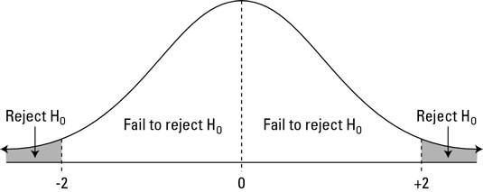
In one-tailed, we will only check for either greater or less (depending on the alternative hypothesis defined) than the probability of mean value. If our null hypothesis is true, we will observe a difference of 1.64 or -1.64 standard error or greater based on the 'right tail' or 'left tail test only 5 out of 100 times. We reject our null hypothesis if our result falls in the shaded range shown in the diagram above, depending on whether the left or right tail test is performed.

NOTE: The critical values of 1.64 used above for one tailed test is figured out using one tailed and two tailed z-score table.

But in a two-tailed test, we need to check the possibility of the weight of passengers being higher and lower as well. Therefore, we will reject the null hypothesis if our sample of passengers has a mean weight significantly higher or lower than the participants' mean weight at athlete completion. We will reject our null hypothesis if 2.5 times out of 100, the mean weight of passengers is either greater or less than the mean weight of participants from athlete competition.

Therefore our testing differs based on the definition of the alternative hypothesis.

Errors

So far, it is evident that the value we will choose for the significant value strongly correlates with the outcome. If it's not, please continue reading. It would lead to an error where we reject the null hypothesis, which is true, or we don't reject the null hypothesis when it is false. Based on this, the error while performing hypothesis testing is divided into two different types:

• Type I error
• Type II error

Type I error is where we reject the null hypothesis, which is true.
E.g., Let's go back to our court example where the null hypothesis is defined as a defendant is not guilty. If we relax a threshold (or, in other words, set a low significance level as 0.1), it will make sure that more criminals go to jail and more innocent will go to jail as well.

Type II error is where we don't reject the null hypothesis when it is false.
E.g., we don't want to send innocent defendants to jail. Now, if we set our threshold high, we will be more likely to fail to reject the null hypothesis that ought to be rejected. If we require five eyewitnesses to convict, many guilty defendants will be set free, but of course, a few innocent will go to prison.

Therefore, I have said earlier that it is advisable to set the significance level before starting the experiment to avoid any potential biases.

Different Statistical tests

In our above analysis, we assumed that our data distribution follows normal distribution; therefore, we used the Z-test and figured out the critical values to perform the hypothesis testing. But this may not be true for every use case we will be working on. We may have different forms of data having different distributions and characteristics. So what are the alternatives that we have?

T-distribution test is a good alternative. It is used whenever the standard deviation of the population is unknown. For sample size ≥ 30, the T-distribution becomes the same as the normal distribution and the output values and results of both t-test and z-test are the same for sample size ≥ 30.

Next, we have two samples that are similar to the Autism example shown above. This test further has two types which include Two-sample mean test - unpaired and a Two-sample mean test - paired. Or once can also use A/B Testing.

Further, there is a Two-sample proportion test test available if we have categorical data. It is used when your sample observations are categorical, with two categories.

The post Understanding Popular Statistical Tests To Perform Hypothesis Testing Is Not Difficult At All! covers technical ways to carry out hypothesis testing using Python programming language. I acknowledge the post is lengthy, maybe bookmark the post and read it once again in your free time to fully grasp the knowledge and depth. I hope it is helpful, and your concept on hypothesis testing is super clear.