Hierarchical clustering algorithm in Python

In the previous post, Unsupervised Learning k-means clustering algorithm in Python we discussed the K Means clustering algorithm. We learned how to solve Machine Learning Unsupervised Learning Problem using the K Means clustering algorithm.

If you don't know about K Means clustering algorithm or have limited knowledge, I recommend you to go through the post.

In this post, we will be looking at the Hierarchical Clustering algorithm which is used to solve the Unsupervised Learning problem. As the name suggest this algorithm is also used to solve clustering unsupervised Learning problem.

Let's get started.

Hierarchical Clustering

One of the biggest challenges with K Means is that we need to know K value beforehand. The hierarchical clustering algorithm does not have this restriction. The hierarchical clustering algorithm groups together the data points with similar characteristics. There are two types of hierarchical clustering:

1. Agglomerative: Involves the bottom-up approach. We start with n distinct clusters and iteratively reach to a point where we have only 1 cluster, in the end, it is called agglomerative clustering. 
2. Divisive: Involves the top-down approach. We start with 1 big cluster and subsequently keep on partitioning this cluster to reach n clusters, each containing 1 element, it is called divisive clustering.

In this post, we will be discussing Agglomerative Hierarchical Clustering.

Agglomerative Hierarchical Clustering

Agglomerative Hierarchical Clustering is the technique, where we start treating each data point as one cluster. Then we start clustering data points that are close to one another. We repeat this process until we form one big cluster.

The steps in hierarchical clustering are:

1. Calculate the NxN distance (similarity) matrix, which calculates the distance of each data point from the other.
2. Each item is first assigned to its own cluster, i.e. N clusters are formed.
3. The clusters which are closest to each other are merged to form a single cluster.
4. The same step of computing the distance and merging the closest clusters is repeated till all the points become part of a single cluster.

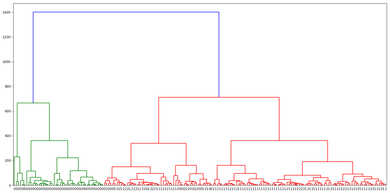
We can visually explore the mentioned clustering using Dendrograms (Inverted tree-shaped structure). Dendrograms are a great way to illustrate the arrangement of the clusters produced by hierarchical clustering. Let's plot one of the dendrograms and see the hierarchical clustering in action:

from scipy.cluster.hierarchy import linkage, dendrogram
from sklearn.datasets import load_wine
import matplotlib.pyplot as plt

data = load_wine()
X = data.data
y = data.target

plt.figure(num=None, figsize=(20, 10), dpi=80, facecolor='w', edgecolor='k')

mergings = linkage(X, method='complete')

dendrogram(mergings, labels=y, leaf_rotation=0, leaf_font_size=10)
plt.show()

OUTPUT:

Method argument in linkage function is used to specify the technique used to measure the distance between two clusters. There are the following techniques which we can use to find the distance between clusters:

• single: The distance between 2 clusters is defined as the shortest distance between points in the two clusters
• complete: The distance between 2 clusters is defined as the maximum distance between any 2 points in the clusters
• average: The distance between 2 clusters is defined as the average distance between every point of one cluster to every other point of the other cluster.
• weighted
• centroid
• median
• ward

NOTE: Different Linkage method results in different hierarchical clustering.

Observations:

1. In the example shown above, we are using the dendrogram function from the scipy package to generate the visualization.
2. We are using a complete method to create a linkage.
3. The height of dendrograms specifies the max distance between the merging clusters. In the plot, it is represented on the y-axis.

Once we have dendrograms plotted, the longest vertical distance without any horizontal line passing through it is selected and a horizontal line is drawn through it. The number of vertical lines this newly created horizontal line passes is equal to the number of clusters. Consider a graph shown below (It is the same graph which is generated from the above example):

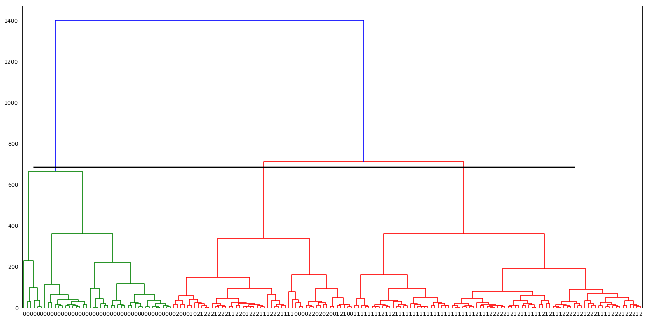The horizontal line drawn in black is the threshold that defines the minimum distance required to be a separate cluster.

Now that we have an understanding of dendrograms. It's time to take one more step and group the data into the clusters. Let's continue with the example to see clusters created in action:

import matplotlib.pyplot as plt  
from sklearn.cluster import AgglomerativeClustering
from sklearn.datasets import load_wine

data = load_wine()
X = data.data
y = data.target

cluster = AgglomerativeClustering(n_clusters=3, affinity='euclidean', linkage='ward')  
cluster.fit_predict(X)  

print(cluster.labels_)

plt.scatter(X[:,0],X[:,-1], c=cluster.labels_, cmap='rainbow')  
plt.show()

Output:

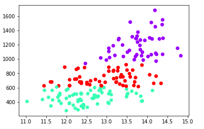
With this, we have successfully found a pattern in our unlabelled dataset.

Is there more? Yes, one last thing before we conclude Agglomerative Hierarchical Clustering. We can also extract out intermediate clusters created.

For e.g., As you can see in dendrogram shown below, What if I want to extract the below cluster:

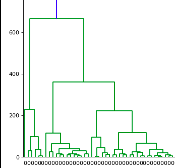
Yes. I can do this by choosing the height on the dendrogram. As you know y-axis on the dendrogram represents the distance between merging clusters. If we want to see the cluster in which data points are grouped to form a specific height we can do this using the fcluster function. Let's look at an example shown below:

import pandas as pd
from scipy.cluster.hierarchy import fcluster
from sklearn.datasets import load_wine

data = load_wine()
X = data.data
y = data.target

mergings = linkage(X, method='complete')

labels = fcluster(mergings, 700, criterion='distance')

df = pd.DataFrame({'labels': labels, 'varieties': y})

ct = pd.crosstab(df['labels'], df['varieties'])

print(ct)

NOTE: The labels represented start from index 1 not from index 0.

Dendrograms looks useful. Don't they?

Limitations

1. Computing the distance of each point from every other point is time-consuming and needs a lot of processing power.

Summary

In this post we learned about:

1. What are hierarchical clustering and its types?
2. We discussed Agglomerative Hierarchical Clustering
3. We learned how to generate dendrograms
4. Various methods that we pass to the linkage method to calculate the distance between the clusters
5. We generated a model with Agglomerative Hierarchical Clustering and saw a pattern by plotting to scatter plot
6. We saw how to extract out intermediate clusters using the fcluster function

In the next post, we will be learning about Divisive Hierarchical Clustering. Please let me know what you think about the post in the comment section below.