Diving Deep into Topic Modeling: Understanding and Applying NLP's Powerful Tool

In the vast sea of digital information, making sense of unstructured text data has become a paramount challenge. In this blog post, we will embark on a journey to unravel the mysteries of Topic Modeling, delving deep into its applications, inner workings, and the transformative impact it can have on understanding, organizing, and extracting meaning from large volumes of text.

Topic Modeling stands as an invaluable asset in the realm of data science, especially for deciphering the underlying themes in a collection of documents. Whether you're a seasoned data scientist or a curious enthusiast, this post will help explore how Topic Modeling can be harnessed to reveal the latent patterns within textual data, offering a key to unlocking valuable insights.

Before we start developing how one can achieve a task of topic modeling, it is important to understand the concept of aboutness. Let's proceed and understand this first.

Aboutness

When machines are analyzing text, we not only want to know the type of semantic associations (Two types of semantic associations is-a and is-in are discussed in the post, Building Block of Semantic Processing: Interpret the meaning of the text) but also want to know what the word or sentence is about. For example, let us consider a sentence "Croatia fought hard before succumbing to France's deadly attack; lost the finals 2 goals to 4."

In the above text which is about football (it could be about other sports such as hockey as well, but let’s keep things simple and assume it’s about football) but has no word 'football' in the text then we want the machine to detect the game of football, then we need to formally define the notion of aboutness.

One way is to detect that the game is football by defining semantic associations such as "Croatia" is-a "country", "France" is-a "country", "finals" is-a "tournament stage", "goals" is-a "scoring parameter" and so on. By defining such relationships, we can probably infer that the text is talking about football by going through the schema. However, this approach will require a lot of searches for such a simple sentence. And, even if we search through the schema, it doesn’t mean we’ll be able to decide that the game is football.

This leads us to define the third type of semantic association which is aboutness. It is about the relevance between the concepts and other concepts (or a group of concepts). For example, {insulin, hypertension, and blood sugar} are collectively "about" diabetes. Therefore, to understand the 'aboutness' of a text means to identify the ‘topics' being talked about in the text.

What makes this problem hard is that the same word (e.g. China) can be used in multiple topics such as politics, the Olympic games, trading, etc.

Topic Modeling

Topic modeling is an unsupervised learning problem which is the art and science of identifying 'latent topics' in text. The topic modeling task is to infer the topics being talked about in a given set of documents.

But the question is, why topic modeling, and how one can use this concept to solve business problems?

Let us consider an example, say a product manager at Amazon who wants to understand what features of a recently released product (say Amazon Alexa) customers are talking about in their reviews. Say the goal is to identify that 50% of people talk about the hardware, 30% talk about features related to music, and 20% talk about the packaging of the product. That would be pretty useful and cool, right? 

Similarly, say we have a large corpus of scientific documents (such as research papers), and we want to build a search engine for this corpus. Imagine if there is a way to infer that a particular paper talks about 'topics' such as diabetes, cardiac arrest, obesity, etc.  Doing a topic-specific search will become easier. To build such applications we use topic modeling. 

The topic by definition is the main idea discussed in the text. But how exactly do we define topics? A topic is usually a distribution over words. It is also possible that a given document refers to multiple topics.

The input to a topic model is the corpus of documents, For example, a set of customer reviews, tweets, research papers, books, etc. There are two outputs of a topic model which include the distribution of topics in a document and the distribution of words in a topic.

Let's understand this further. In the following figure, the first matrix is the probability distribution of words in a topic (topic-term distribution), while the second matrix is the distribution of topics in a document (document-topic distribution). 

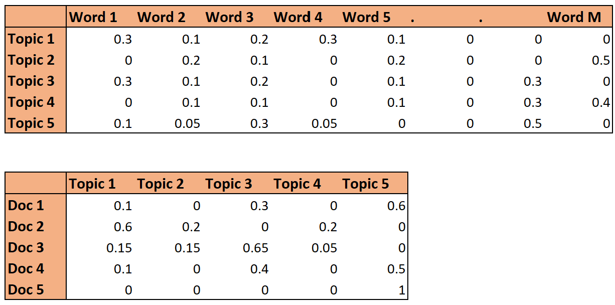
A topic is a distribution over words, i.e. each word has a certain weight in each topic (which can be zero as well) as shown in the diagram above. But is that the only way to define topics? What are the other ways we could define topics, and what are some pros and cons of them?

Defining Topic as a word

Let us consider an oversimplified definition of topic modeling and consider every term or word as a topic. We will see the cons of this approach as it is not ideal to define a topic in this way.

There are two major tasks in topic modeling or generating a topic for a given text corpus which are defining the topic and estimating the coverage. The first task is simply estimating the topic-term distribution. In this case, we have defined each topic as a single term.

But the more challenging task is estimating the coverage of topics in a document, i.e. the document-topic distribution. where coverage is defined as:

Coverage = the frequency of topic j in document i / ∑j (the frequency of topic j in document i )

This simply means that we are calculating term frequencies, where we are counting the number of times a topic (which is defined as a word in a document for our oversimplified case) appeared in a document over all the topics appearing in the document.

Some problems with defining topics as a single term are:

1. Polysemy: If a document has words having the same meaning (such as lunch, food, cuisine, etc.), the model would only choose one word (say food) as a topic and ignore all the others.
2. Word sense disambiguation: Words with multiple meanings such as 'stars' would be incorrectly inferred as representing only one topic, though the document could have both topics (movie stars and astronomical stars)

Let's consider an example where we have two topics 'stars' for a text about astronomy and 'film' for a text about movies. Now consider the example sentence "The stars are out tonight at the 19th annual Film Awards"

Here both stars and films are equal in frequency and stars are also talking about the topic of movies and not astronomy. Since words can have different meanings, therefore we have to do better as the term as a topic approach doesn't fit well.

Though it doesn't solve the problem it is still good to know as it helps in appreciating the concept of topic modeling and the complexity involved. Thus, we need a more complex definition of a topic to solve the problem of polysemy and word sense disambiguation.

Defining Topic as a distribution over vocabulary

We solve this by considering the topic as a distribution over a vocabulary as we have seen earlier briefly. There are multiple advantages of defining a topic as a distribution over terms instead of simply defining every term as a topic.

Primarily, now words can have different weights in different topics which allows subtle differences in topics i.e., P(w | topic). Also, word sense disambiguation is resolved depending on the topic. Let us consider an example with two topics - 'magic' and 'science'.

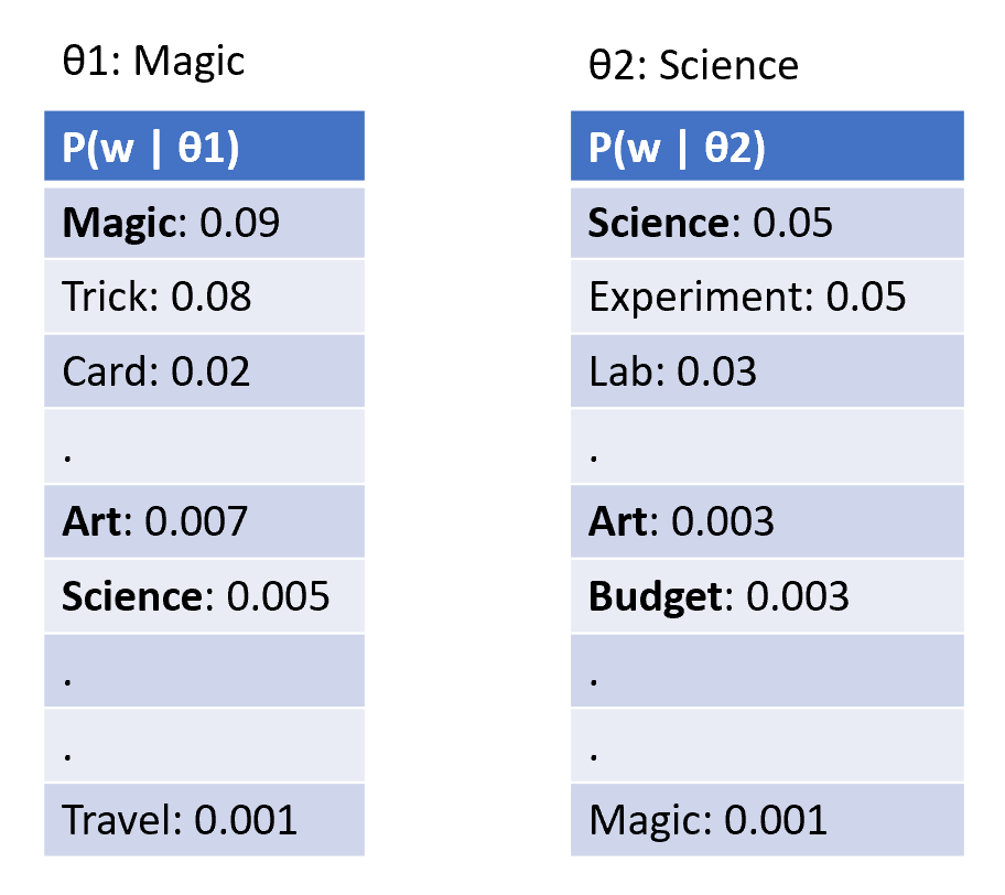
The term ‘magic’ has a very high weight in the topic 'magic' and a very low weight in the topic 'science'. A word can have different weights in different topics. We can also represent more complex topics that are hard to define via a single term.

There are multiple models through which we can model the topics in this manner. Let's first briefly study the simple approach of matrix factorization for topic modeling.

Matrix Factorisation-based Topic Modelling

One possible approach for topic modeling is matrix factorization. However, this technique is not commonly used for topic modeling. Having an understanding of this technique gives an interesting viewpoint and helps draw motivation for more sophisticated techniques such as PLSA and LDA which we will discuss later in the post.

The technique is about applying SVD on the document-term matrix. We are given a metric, M x V which can be factorized as M x K, K x K, and K x V. Where M is the number of documents, V is vocabulary, and K is the number of topics.

We know that the goal is to find a matrix that gives the relation of documents to the topic and another matrix that gives the relation to topics to word. i.e., M x V and K x V respectively is exactly what matrix factorization using SVD gives us.

What are the drawbacks to the approach?

In PCA we define that principal components (which in this case are topics) should be orthogonal to each other and further the strength of principal components should be in decreasing order. Now, we have to ask ourselves does this make sense here? May not be in most cases. So, we need a better approach to solve the problem.

Explicit Semantic Analysis (ESA)

ESA is another unpopular technique used for topic modeling, but worth discussing, where the topics are represented by a 'representative word' that is closest to the centroid of the document. Say we have N Wikipedia articles as documents and the total vocabulary is V. We first create a TF-IDF matrix of the terms and documents so that each term has a corresponding TF-IDF vector.

Now, if a document contains the words (For example, sugar, hypertension, glucose, saturated, fat, insulin, etc.) each of these words will have a TF-IDF vector. The centroid of the document will be computed as the centroid of all these word vectors. The centroid represents the average meaning of the document in some sense. Now, we can compute the distance between the centroid and each word, and let’s say that we find the word vector of 'hypertension' is closest to the centroid. Thus, we conclude that the document is most closely about the topic 'hypertension' for the example words.

Note that it is also possible that a word that is not present in the document is closest to its centroid. For example, say we compute the centroid of a document containing the words 'NumPy', 'cross-validation', 'preprocessing', 'overfitting', and 'variance', it is possible that the centroid of this document is closest to the vector of the term 'machine learning' which may not be present in the document.

Having an understanding of the some of basic algorithms such as Matrix Factorisation-based Topic Modelling or Explicit Semantic Analysis that can be used for the task of topic modeling, next, let us understand the popularly used probabilistic models approach for topic modeling.

Probabilistic Model

We will next discuss the basic idea of generative probabilistic models in the context of topic modeling. Informally speaking, in generative probabilistic modeling, we assume that the text corpus is generated through a probabilistic model. Then, using the observed data points, we try to infer the parameters of the model which maximize the probability of observing the data.

For example, we can see POS-tagged words as data generated from a probabilistic model such as an HMM. We then try to infer the HMM model parameters which maximize the probability of the observed data.

Assumptions made for the topic modeling using the probabilistic approach:

• The words in documents are assumed to come from an imaginary generative probabilistic process.
• The order of words in a topic is assumed to be unimportant.
• The process to generate a document is to draw words one at a time.

Before we go ahead and discuss probabilistic models, let's define the plate notation that we are going to use throughout over probabilistic model discussions.

Plate Notation

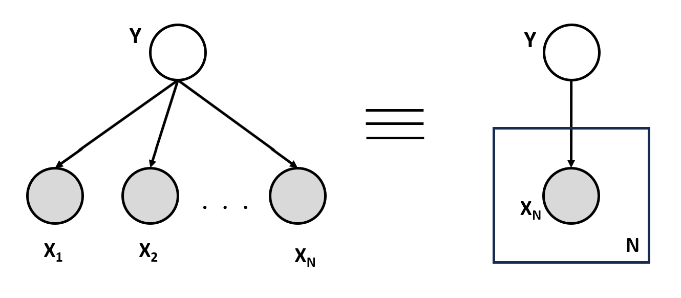
A concise way of visually representing the dependencies among model parameters. It's a graphical model where:

• Nodes are random variable
• Edges are dependencies: X1 depends on Y, X2 depends on Y, etc.
• Observed variables are shaded, and unobserved ones are not
• Plates represent the repetitive structure

Refer to the diagram shown below:

Unigram Model

Moving forward, the Unigram model is one such simple probabilistic model that can be used for topic modeling where word is drawn one at a time assuming that words in a sentence are independent of each other. Though the unigram model which is just looking at the words, is not very useful for language modeling it is sufficient for the problem of topic modeling.

There are various models better than the simple unigram model in which we can extract topics from the text such as PLSA (Probabilistic Latent Semantic Analysis) and LDA (Latent Dirichlet Allocation). Let's discuss them next and start with PLSA.

Probabilistic Latent Semantic Analysis (PLSA)

Earlier we have gone through the topic modeling technique called ESA where 'explicit' indicates that the topics are represented by explicit terms such as hypertension, machine learning, etc., rather than 'latent' topics such as those used by PLSA. It is a probabilistic technique that can be represented as a graphical model having the random variables documents d, topics C, and words W. The number of topics C is a hyperparameter specified at the start of the computation.

First, we fix an arbitrary number of topics which is a hyperparameter (For example, let's say we decided that there are 20 topics in all documents). The model assumes that each document is a collection of some topics and each topic is a collection of some terms.

For example, a topic \(t_1\) can be a collection of terms (hypertension, sugar, insulin, ...), \(t_2\) can be (NumPy, variance, learning, ...), etc. The topics are not given or defined, we are only given the documents and the terms.

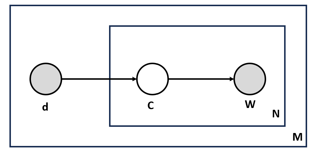
In the diagram shown above, we read from the outer plate to the inner plate, where M represents the document, d is the document index which points to the N times box which represents N such words W appearing in the document, for every single word there is a topic represented as C (also called as latent).

Only document d and words in document W are observed and topic C is not observed and is not shaded in the diagram shown above. The probability of observing a document and word is given as:

$$P(W, d) = P(d)P(W|d)$$

This is according to the Bayes’ rule which relates joint and conditional probability as P(A, B) = P(A|B).P(B) = P(B|A). P(A).

Now, P(w|d) represents the probability that a word w is drawn given a document d. But in the generative process, we have assumed, that words do not come from documents, but rather, words are drawn from topics drawn from documents. Therefore P(W|d) can be written as,

$$P(W, d) = P(d)P(W|d) = P(d)\sum_CP(C|d).P(W|C)$$

Our defined model assumes that words are generated from topics, which in turn are generated from documents. Therefore we are summing over all the topics to get the probability of P(W|d). In the equation above, P(C|d) which is the topic distribution given the document, and P(W|C) which is the term distribution given the topic are modeled as multinomial distribution.

Before moving forward, let’s first understand how P(C|d) and P(W|C) are modeled using a multinomial distribution.

Multinomial Distributions

The multinomial distribution is a generalization of the binomial distribution. For example, conducting an experiment that generates a binomial distribution is tossing a coin N times, where each coin tossed results in a head or a tail. But in a multinomial distribution, each toss (still independent of other tosses) can have more than two outcomes.

Another example experiment that generates a multinomial distribution is rolling a k-sided die (with digits from 1,2,...k) N times. Now, each roll of the die can result in k outcomes with probabilities \(p_1\),\(p_2\)...\(p_k\). Since in each roll of the die, one of the k numbers should appear, it is evident that:

$$\sum_kp_i = 1$$

When we do N rolls of the die, we will get N digits from 1 to k as the outcomes where digits 'i' which have a higher probability \(p_i\) will appear more frequently than those with low \(p_i\). This is how we can define the multinomial distribution. To understand more about distributions refer to the post, A complete guide to the Probability Distribution.

Using Multinomial Distribution for Topic Modeling

Let's now see how the multinomial distribution is represented mathematically and used in the context of topic modeling. Consider our k-sided die and say that we roll it N times. Let the random variable \(X_i\) denote the number of times the digit 'i' appears, i.e. \(X_1\) represents the number of times 1 appears, \(X_2\) represents the frequency of 2, and so on.

The probability that the digit 1 appears \(x_1\) times, 2 appears \(x_2\) times.... digit k appears \(x_k\) times is given by the expression below. Also, note that since there are total N tosses, the number of times each digit (each side of the die) appears should add up to N, i.e.,

$$\sum x_i = N$$

The random variable (now a vector) X=(X1, X2, X3...Xk) is said to follow a multinomial distribution. The probability of this random variable taking the values (x1,x2....xk) is given by:

P(X1=x1, X2=x2,...,Xk=xk)=n!x1!x2!......xk!px11px22......pxkk

To take an example, say we have a 3-sided die (k=3) with the letters A, B, and C on each side which occur with probabilities (0.2, 0.5, 0.3) respectively. If we roll the die N=4 times, the probability of A, B, and C appearing 1, 1, and 2 times respectively is given by:

P(A=1, B=1, C=2)=4!(1!1!2!)(0.21)(0.51)(0.32)

Now let's see how the 'topic-term distribution' can be modeled as a multinomial distribution (more accurately, it is modeled as a Dirichlet distribution which we will understand later in the post).  Let us clarify this with the help of an example.

Say we have k terms representing a topic c = 'magic' (terms such as ‘magic’, ‘black’, ‘cards’ … etc.). We can imagine a k-sided die with each side containing a term w and having some probability P(W|C). Also, say we want to generate N terms from this topic.

This can be done by rolling the k-sided die N times where each roll generates a term (according to the probability P(W|C) ). The random variable X is a vector whose values represent the number of times a particular word appears in a topic C (say 'magic'), i.e. X=(magic=6,black=4,…wk=xk).

Similarly, a document can be seen as a multinomial distribution over the topics i.e., 'document-topic distribution' where a k-sided die is a 'document' with each side representing one 'topic' (along with the 'probability of the topic' in the document). For example, the random variable \(X=(t_1=4,t_2=10,t_3=14,t_4=16,t_5=11)\) represents the number of times each topic occurs in the document (i.e. topic-1 occurs 4 times, topic-2 occurs 10 times and so on).

This is how both P(C|d) and P(W|C) are modeled using a multinomial distribution.

Inference task for PLSA

Coming back to our discussion of PLSA, document d contains each topic with some probability (document-topic distribution), and each topic contains the W words with some probability (topic-term distribution). The inference task is to figure out the d x C document-topic probabilities and the C x W topic-term probabilities. In other words, we want to infer Cd + WC parameters.

The basic idea used to infer the parameters, i.e. the optimization objective, is to maximize the joint probability p(W, d) of observing the documents and the words (since those two are the only observed variables). We can estimate the Cd + WC parameters using the expectation maximization (EM) algorithm. Let's understand in detail about the expectation-maximization algorithm next.

Expectation Maximisation (EM) Algorithm

PLSA tries to maximize the posterior probability P(C | d,W) where we find the probability of observing a topic given a document and words in the document using the Expectation Maximisation (EM) algorithm assuming there is k number of topics C.

The EM algorithm works in two steps which include E-step calculation and M-step calculation. Let's understand the two steps involved in the EM algorithm.

E-step Calculation

Here we calculate the probability of the topic given the word and document. We start with the random values for the missing parameters.

$$P(C|d,W) = {P(C)P(d|C)P(W|C) \over \sum_CP(C)P(d|C)P(W|C)}$$

M-step Calculation

We now know the P(C|d,W) which we just computed from the previous step. We use this with the frequency of the document and word to calculate:

$$P(W|C) \propto \sum_Dn(d,W)P(C|d,W)$$

$$P(d|C) \propto \sum_Wn(d,W)P(C|d,W)$$

$$P(C) \propto \sum_d\sum_Wn(d,W)P(C|d,W)$$

We repeat the M-step where we update the hypothesis and the E-step where we update the variables again and again until the solution is converged. In this way, we can estimate the variables needed for the PLSA algorithm.

Example Demonstrating the use of PLSA

Let's go through an example that demonstrates an interesting way to use PLSA. We have users who are reading certain articles. And the task is to identify user's interests based on the articles they are reading. How we can solve this problem using topic modeling?

Let's assume we have done topic modeling with two topics as parameters and classified each article into one of the topics. Now articles or documents will be distributed over the topic and words will be distributed for a given topic as shown in the diagram below.

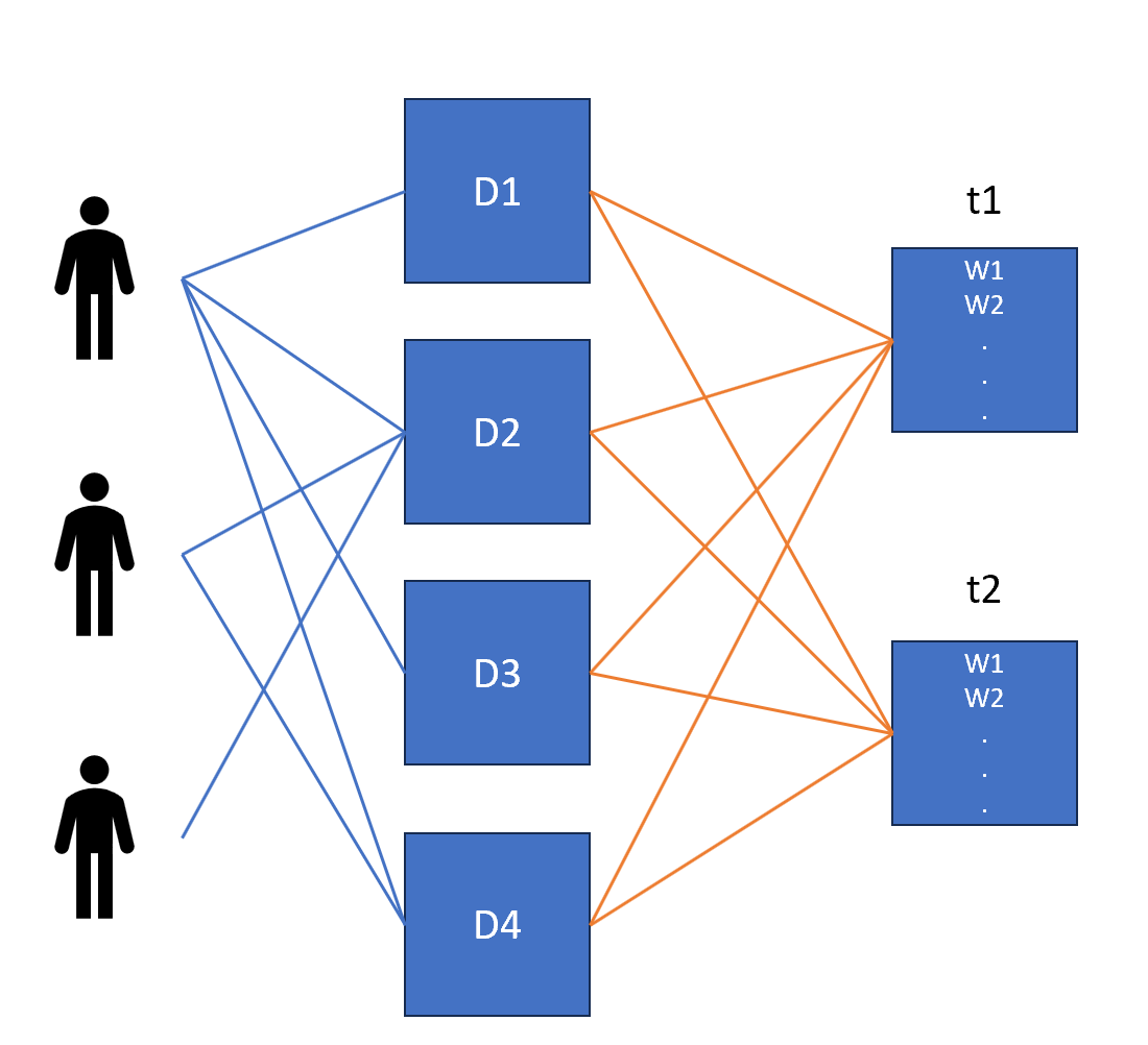
Now, in this way, we can understand a topic a user is interested in and the word distribution among the topics. PLSA models topics as a distribution over terms and documents as a distribution over topics. The parameters of PLSA are all the probabilities of associations between documents-topics and topics-terms which are estimated using the expectation-maximization algorithm as we have discussed above.

Drawbacks of PLSA

The major drawback of PLSA is that it has lots of parameters (Cd + WC) that grow linearly with the documents d. Although estimating these parameters is not impossible, it is computationally very expensive. 

For example, if we have 10,000 documents (say Wikipedia articles), and 20 topics, and each document has an average of 1,500 words, the number of parameters you want to estimate is 1,500*20 + 20*10,000 = 230, 000.

PLSA is also prone to overfitting on small datasets because it has a large number of parameters that can overfit. Let's understand another approach that is widely used in the industry called LDA which is an extension of the PLSA algorithm.

Latent Dirichlet Allocation (LDA)

LDA (Latent Dirichlet Distribution) is an alternative topic model that solves the problem of large parameter estimation with the PLSA technique. Unlike PLSA, LDA is a parametric model, i.e. we do not have to learn all the individual probabilities. Rather, we assume that the probabilities come from an underlying probability distribution (Dirichlet distribution) which can be modeled using a handful of parameters.

For example, the normal distribution is parameterized by only two parameters i.e., the mean and the standard deviation. Modeling data using this distribution (such as the age of N people) means estimating these two parameters. Similarly, in LDA, we assume that the document-topic and topic-term distributions are Dirichlet distributions (parameterized by some variables), and we want to infer these two distributions.

Understanding LDA Modeling

LDA is specified as a Bayesian model where parameters are random variables with some known prior distributions. Unlike PLSA where we need to find all the parameters, in LDA we just need to find the parameters that form the distribution instead of finding all the parameters.

LDA can also be regularized in the sense that we can control the plugs that define the topic for the given documents based on prior knowledge.

We have defined a generative process in PLSA as each document is a distribution of topics and each topic is a distribution of terms. Next, let us define the generative process for LDA. Refer to the example diagram shown below.

The generative process of LDA is a probabilistic model that describes how a corpus of documents is generated. It assumes that each document is a mixture of latent topics, and each topic is a distribution over words. For each document d in the corpus we choose document-topic distribution from Dirichlet distribution and for each word in the document, we choose a topic from the earlier chosen document-topic distribution and choose the word W from the chosen topic.

The generative process assumes that each document is generated independently of the others, and the same set of topics is used across all documents. By assuming a generative process for the data, LDA allows us to infer the latent variables that generate the observed data and discover the underlying topics in the corpus.

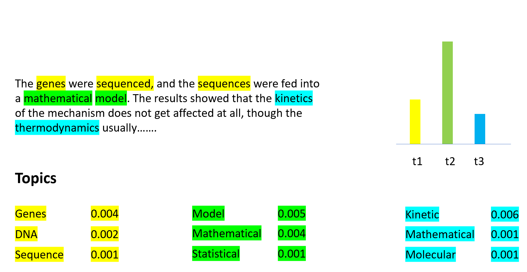
In the diagram shown above, we are given the topic distribution in a given document (represented as a bar graph in the diagram above) i.e., document-topic distribution, and also distribution of words in a given topic is also given i.e., topic-term distributions. Both distributions come from the Dirichlet distribution.

Parameters of the LDA Model

Let's now understand the various parameters involved in LDA modeling using a plate diagram as shown below. There are two Dirichlet parameters alpha and eta. The alpha is a parameter of the Dirichlet distribution which determines the document-topic distribution, while eta is the parameter that determines the topic-term distribution.

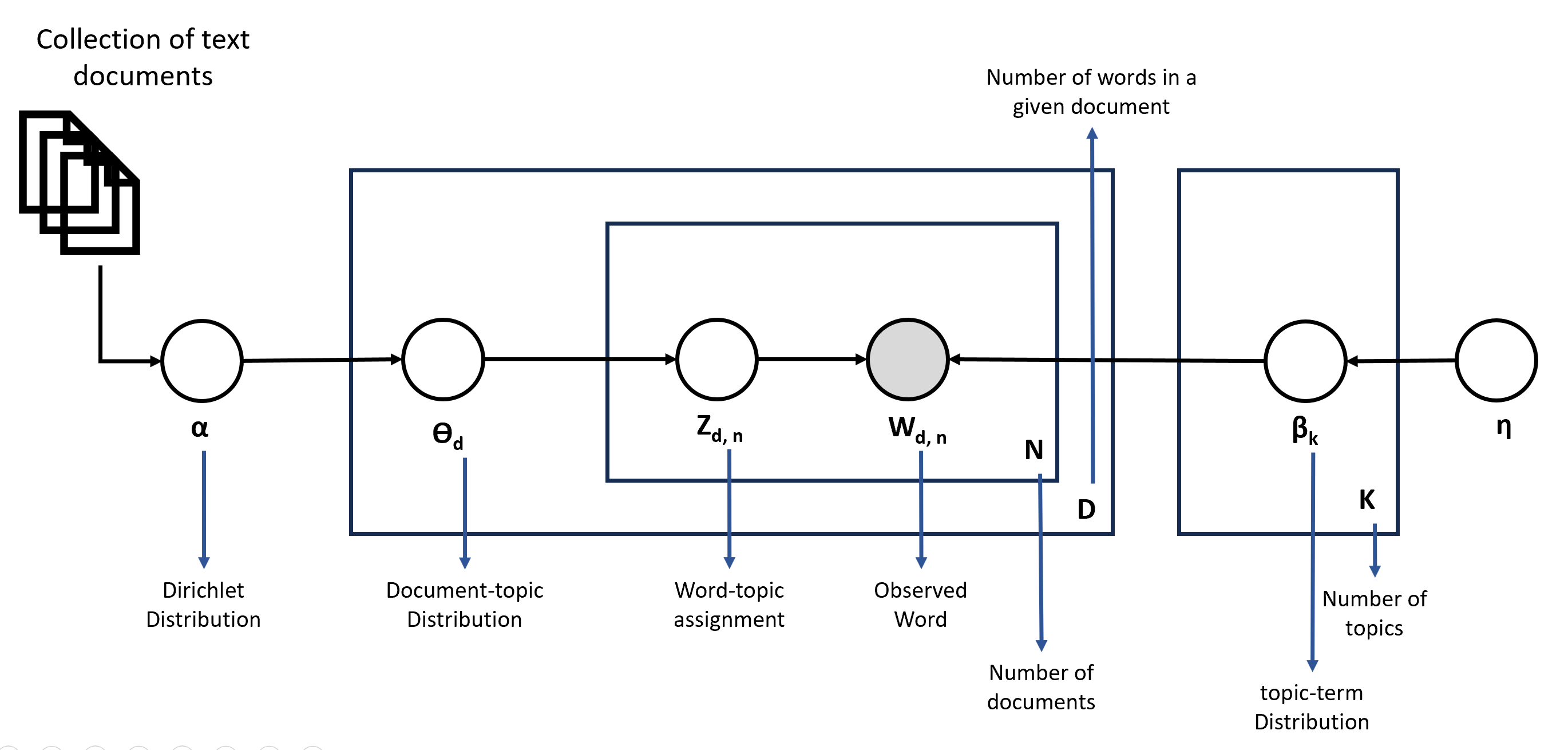
Beta and theta are the two Dirichlet distributions used in LDA. The high alpha value represents that all topics are given equal weightage in the document.

\(\theta_d\) is the topic distribution over the given document d (which is coming from the Dirichlet distribution characterized by alpha). From the chosen topic distribution for a given document d, we next need to determine the topic for every word in the document. \(Z_{d,n}\) is a topic assignment for the words in the word position in the document. It is a number from 1 to K assuming there are K topics. Once the topic is assigned to the word (chosen topic is coming from \(\beta_k\) which is the term distribution for the document d. The K plate represents that for each topic we have the word distribution which is characterized by eta.), we go next and pick a word from the assigned topic for a given word W in the document d. It is represented as \(W_{d,n}\).

In the above shown diagram only word shaded in color is observed and all other parameters are derived variables. Also, beta and theta are the two Dirichlet distributions used in LDA that control the topic modeling. The high value of alpha means that the document will be represented by many topics, hence topics would be given equal weight, and the same is true with eta.

Before going forward, let us understand what is Dirichlet distribution as we have been using this a lot throughout the discussion of LDA.

Understanding Dirichlet Distribution

So far we have an understanding that the document-topic and topic-term distributions are modeled as a parametric distribution called the Dirichlet. Also, the Dirichlet distribution is parameterized by a variable 'alpha'. By specifying a particular value of alpha, we define the rough shape of the Dirichlet distribution (similar to when we define μ and σ to get the shape of a Gaussian distribution).

In the PLSA section, we have defined how document-topic and topic-term distribution is modeled using a multinomial distribution and we have defined document-topic and topic-term distribution as the number of times a topic appears in a document or the number of times a word appears in a topic respectively.

Now, let's modify this, and rather than each topic taking an integer value, we here want it to take a value between 0 and 1, i.e. we want each topic \(t_1,t_2,...t_k\) to appear with probabilities \(p_1,p_2...p_k\). Similarly, we want to model the topic-term distribution such that each term \(w_1,w_2...w_k\) appears with some probability \(p_1,p_2...p_k\) in a topic.

The two multinomial distributions thus obtained, where the random variable X represents the probability of occurrence of a topic in a document/term in a topic, is a Dirichlet distribution. In general, a Dirichlet distribution is similar to the multinomial distribution that describes k>=2 variables \(x_1,x_2...x_k\) with each \(x_i\) being between [0,1] and \(\sum x_i = 1\).

The probability distribution function or PDF for Dirichlet distribution is defined as:

$$f(x_1, . . . .,x_K; \alpha_1, \alpha_2, . . . , \alpha_K) = {1 \over B(\alpha)}\prod^K_{i=1}x_i^{\alpha_i-1}$$

The Dirichlet is parametrized by a vector \(\alpha = (\alpha_1, \alpha_2, ..., \alpha_k)\). The individual alphas can take any positive value (i.e. not necessarily between 0 and 1), though the x'is are between 0 and 1 (and all x'is add to 1 since they are probabilities). When all alphas are equal, i.e. \(α=α_1=α_2=...=α_k\), it is called a symmetric Dirichlet distribution. In LDA, we assume a symmetric Dirichlet distribution and say that it is parameterized by alpha.

Let’s visualize the Dirichlet using an example of document-topic Dirichlet distribution. Say we have 3 topics \((t_1, t_2, t_3)\) in all your documents.  Each document will have a certain topic (Dirichlet) distribution.

Let’s say that the first document \(d_1\) has the topic distribution \((t_1=0.2,t_2=0.6,t_3=0.2)\), the document \(d_2\) has the distribution \((t_1=0.5,t_2=0.2,t_3=0.3)\) and so on till document \(d_n\). Also, consider an extreme case that the document \(d_100\) has only one topic \(t_1\), and thus, has the distribution \((t_1=1.0,t_2=0.0,t_3=0.0)\).

Now, it will be nice to be able to plot the topic distributions of all these documents. The way to do that is by using a simplex as shown below. 

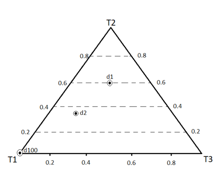
The vertices represent the three topics which include \(t_1\), \(t_2\), \(t_3\). The closer a point is to a vertex, the more that vertex’s 'weight'. For example, the document \(d_100\) having all its weight on \(t_1\) is a point on the vertex \(t_1\). The point representing document \(d_1=(t_1=0.2,t_2=0.6,t_3=0.2)\) is closer to \(t_2\) and farther (and equidistant) from \(t_1\) and \(t_3\). Finally, \(d_2=(t_1=0.5,t_2=0.2,t_3=0.3)\) is closest to \(t_1\), slightly close to \(t_3\) and far from \(t_2\).

Now, imagine if we have N=10,000 documents each plotted as a point on this simplex. The shape of this distribution is controlled by the parameter alpha (assuming a symmetric distribution). The four figures below show the different shapes of Dirichlet distributions as alpha varies.

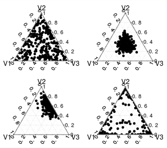
• At alpha=1 (figure-1) the points are distributed uniformly across the simplex.
• At alpha > 1 (figure 2, top-right) the points are distributed around the center (i.e. all topics have comparable probabilities such as \((t_1=0.32,t_2=0.33,t_3=0.35)\)).
• The figure on the bottom-left shows an asymmetric distribution (not used in LDA) with most points close to topic-2.
• At values of alpha < 1 (figure-4), most points are dispersed towards the edges apart from a few which are at the center (a sparse distribution - most topics have low probabilities while a few are dominant). 

Note that when we take a sample from a Dirichlet (such as \(T=(t_1=0.32,t_2=0.33,t_3=0.35)\)), T itself a probability distribution, and hence a Dirichlet is also often called a distribution over distributions.

Having an understanding of how the Dirichlet distribution works, let's come back to our LDA model parameters and figure out an approach on how we can define the document-topic distribution for each document \(\theta_d\), topic-term distributions for every word in a document \(\beta_k\), and topic assignment for the words in the document \(Z_{d,n}\).

There are various approximation methods such as Variational EM, Expectation propagation, Collapsed variational inference, Gibbs sampling, and Collapsed Gibbs sampling for LDA. In this post, we will focus on Gibbs sampling as it is a popular method to estimate the parameters.

Parameter Estimation using Gibbs Sampling

Gibbs sampling is a type of Markov Chain Monte Carlo (MCMC) method that is a commonly used technique in LDA (among many other techniques such as variational EM, expectation propagation, etc.). To perform Gibbs sampling, we need to specify the following steps:

1. Choose an initial value for each variable in the distribution.
2. For each iteration, do the following:
   1. For each variable, update its value by sampling from its conditional distribution given the current values of the other variables.
   2. Store the updated values as a new sample in the sequence.
3. Repeat step 2 until a desired number of samples is obtained or a convergence criterion is met.

It is very similar to the EM technique that we have discussed in PLSA. Here as well initially the joint probability is poor but as we keep on iterating over the joint probability converges. The details of how Gibbs sampling works are out of the scope of this post.

Then we can further perform the document similarity.

Python Code for Topic Modeling using LDA algorithm

Let us understand how we can code the LDA algorithm for topic modeling purposes using gensim implementation. The sample code shown below demonstrates how we can use LdaModel from the gensim package to build an LDA topic model.

lda_model = gensim.models.ldamodel.LdaModel(corpus=corpus,
                                           id2word=id2word,
                                           num_topics=10, 
                                           random_state=100,
                                           update_every=1,
                                           chunksize=100,
                                           passes=10,
                                           alpha='auto',
                                           per_word_topics=True)

We will cover two different examples to find the topics. Consider the first example where a product manager at Amazon wants to understand what features of a recently released product (say Amazon Alexa) customers are talking about in their reviews. The goal is to identify topics such as hardware, music, packaging, etc., and customer opinions.

In the second example, we have considered the Twitter (now called X) dataset related to the demonetization that happened in India and the goal is to again find the topics which can help classify the opinions of the users about demonetization.

Both of these examples are built out thoroughly starting from data preprocessing all the way to identify topics in the datasets. Refer to Jupyter notebook for details.

Summary

In our exploration of Topic Modeling, we've traversed the nuanced landscape of aboutness, seeking to uncover the essence of textual data. From deciphering the inherent themes to understanding the very fabric of language, we've delved into the heart of NLP's formidable tool which is Topic Modeling.

Throughout this post, we've encountered various techniques such as Matrix Factorisation-based Topic Modelling, with its capacity to reveal underlying patterns through matrix decomposition, and Explicit Semantic Analysis (ESA) which provided us with a lens to view documents in the context of a vast semantic space, and Probabilistic Latent Semantic Analysis (PLSA) and Latent Dirichlet Allocation (LDA) acted as guiding lights, offering probabilistic models to unveil the latent topics concealed within our textual troves.